Research Journal of Applied Sciences, Engineering and Technology
Numerical Study on Time Dependent Maxwell Nanofluid Slip Flow over Porous Stretching Surface with Chemical Reaction
Research Journal of Applied Sciences, Engineering and Technology 2020 17: 24-34
Cite This ArticleAbstract
The recent study deals with the numerical analysis of an unsteady Maxwell nanofluid flow passing through a porous stretch surface with slip boundary condition with chemical reaction effect using Buongiorno's mathematical model. The water-based fluid and the gold nanoparticles (Au) are preferred for this study. The similarity transformations are applied to renovate the governing model equations into a set of ordinary non-linear differential equations. The solutions of the coupled non-linear dimensionless equations are numerically decoded using the Nachtsheim-Swigert shooting method together with the Runge-Kutta iterative technique for various values of the flow control parameters. In addition, the built-in function bvp4c of MATLAB is used to enhance the consistency of numerical results. The numerical results are graphically demonstrated and narrated from the physical point of view for the non-dimensional velocity, temperature and concentration profiles, as well as the local coefficient of skin friction, Nusselt number and Sherwood number for different parameters of materials, such as the volume fraction parameter, Deborah number, unsteadiness, slip, stretching, suction and chemical reaction parameters. It is witnessed that the heat transfer rate is widely controlled by the Deborah number for Au-water nanofluid. The outcomes of this analysis clearly indicate the considerable influence of the suction imposed in the model.
Keywords:
Introduction
The low thermal conductivity of traditional heat transfer fluids like water, engine oil and ethylene glycol is a grave limitation in developing the performance, efficiency and solidity of modern engineering equipments. Nanofluids engineered by stably suspending and uniformly dispersing a small amount of nano-sized (between 1 and 100 nm in diameter) ultrafine metallic, nonmetallic or ceramic particles in ordinary heat transfer fluids are the newly invented heat transport fluids containing thermal conductivity to a great extent at low concentration than traditional fluids. This idea of colloidal suspension in regular fluid, as a concept of nanofluid, was first developed by Choi and Eastman (1995). Recent researchers have identified that the replacement of conventional coolants with nanofluids may be advantageous for improving the competence of heat transfer in the nuclear space and engineering, chillers, domestic refrigerators/freezers; and cooling of engine and microelectronics (Sridhara and Satapathy, 2011). As well nanofluids are used as the antibacterial agent in textile industry, water disinfection, medicine and food packaging (Hajipour et al., 2012; Uddin et al., 2016). Moreover, the electromagnetic nanoparticles used to control and operate the nanofluids through magnetic force are playing an important role in biomedical purposes compared to other metal particles, Chiang et al., (2007). Due to the mounting demand for encompassing extraordinary characteristics of providing unique physical and chemical properties nanofluids are receiving significant interest of many scientists and researchers, Emerich and Thanos (2006), Ma et al., (2006), Buongiorno et al., (2008) and Kuznetsov and Nield (2010). As a part of these researches, Buongiorno (2006) composed a precise model to investigate the heat transfer by convection in nanofluids taking into account the effects of Brownian motion and thermophoresis diffusion.
The research on the boundary layer of non-Newtonian fluid flow is the primary focus for the last few decades because of the multiplicity of its practical purposes in technology and industrial processes, for instance in geophysics, petroleum, biomedical and chemical industries, Mushtaq et al., (2016). The characteristics of the non-Newtonian fluid flow are quite unusual compared to Newtonian fluids. The momentum equations of these fluids are particularly nonlinear and the Navier-Stokes equations undoubtedly are not adequate to illustrate the flow of non-Newtonian fluids, Mustafa and Mushtaq (2015). Almost all rheological complex fluids, for example, industrial and biological fluids such as polymer solutions, paints, pulps, fossil fuels, molten plastics, liquid foods, jams and blood demonstrate the non-linear alliance between deformation and stress rates (Bandelli, 1995; Fetecau and Fetecau, 2003). The non-Newtonian fluid models are developed by the researchers involving the constitutive equations tending to be highly nonlinear and are able to predict the rheological characteristics, Tan and Masuoka (2005). These models are mostly categorized into three classes: rate-, differential-and integral-type fluids. The Maxwell fluid model enclosed with viscoelastic material is the simplest subclass of rate-type non-Newtonian fluids. This model is capable to elucidate the characteristics of the relaxation time effect of fluids where the differential-type fluids fail to predict, Gallegos and Mart´ınez-Boza (2010). A revolutionary work done by Harris (1977) portraying 2D flow of Maxwell fluids is promoting the researchers to investigate more possibilities. Following this route, Fetecau et al., (2010) explored the viscoelastic fluid flow by way of fractional Maxwell model subjected to time dependent shear stress. The Maxwell fluid model is reduced into the simple Navier-Stokes relation in the absence of the effect of relaxation time (Sochi, 2010).
Very recent, a number of researchers investigated a choice of parametric effects like Joule heating; heat source and thermal radiation on Maxwell fluid flow passing above a stretching sheet (Abbas et al., 2006; Aliakbar et al., 2009; Abel et al., 2012; Nadeem et al., 2014). The natural porous media are wood, beach sand, limestone, bile duct, sandstone, small blood vessels, gall bladder with stones and the human lung, Nield and Bejan (2006). Hayat and Qasim (2010) explained a pathological situation, for example, the fatty cholesterol distribution in the lumen of coronary artery is equivalent to the fluid flow in a porous surface. Metallic nanoparticles are promising vectors of drug administration to the brain. The common metals used for the administration of drugs in nanoparticles are gold, silver and platinum, due to their biocompatibility. These metallic nanoparticles are used because of their large surface area at volume ratio, chemical and geometric tuning and endogenous antimicrobial properties, Mandal (2017). The silver cations released by the silver nanoparticles can bind to the cell membrane of negatively charged bacteria and increase the permeability of the membrane, thus allowing foreign chemicals to enter the intracellular fluid. The metal nanoparticles are synthesized chemically using reduction reactions, Kumar et al., (2018). For example, silver nanoparticles conjugated to the drug are created by reducing silver nitrate with sodium borohydride with an ionic drug compound. Niu and Li (2014) expressed the fact that the active drug ingredient binds to the surface of silver, stabilizes the nanoparticles and prevents the aggregation of the nanoparticles.
With an objective to describe the flow of blood as a rheological fluid containing nanoparticle drugs that react destructively through blood vessels in the presence of an electromagnetic field, the analysis of unsteady two-dimensional laminar flow of chemically reacted Gold (Au)-water nanofluid passing through the porous stretching surface with the slip boundary condition is executed in this article by applying the Maxwell rheological fluid model.
Mathematical Model
This study was conducted 4 Months before, PhD research work, Dept. of Applied Mathematics, University of Dhaka, Dhaka-1000, Bangladesh.
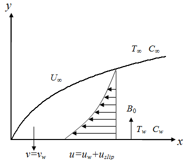
In the present model, a two-dimensional time dependent flow of an electrically conducting non-Newtonian Maxwell nanofluid with magnetic field and chemical reaction effects passing a semi-infinite stretching porous surface with slip boundary condition is considered. If elastic stress is applied to a non-Newtonian fluid, the resulting strain will be time dependent characterized by the relaxation time.
The constitutive equation for a Maxwell fluid (Fetecau and Fetecau, 2003) is:
$ \tau = -p \bf {I} \rm + \bf {S} $
where the Cauchy stress tensor is denoted by $\tau$. And the extra stress tensor $S$ satisfies:
$ \bf S \rm+k\left(\frac{d\bf S \rm}{dt}-\bf {LS}-\bf {SL}\rm ^{tr}\right)=\mu_{0} \bf {A}_\rm{1} $
In which $ \mu_{0} $ is the viscosity, $ k > 0 $ is the relaxation time and the Rivlin-Ericksen tensor $ A_{1} $ is defined through:
$A_{1}=\bigtriangledown V+\left(\bigtriangledown V\right)^{tr}$
The relaxation time for Maxwell fluid is considered by $ k=k_{0}\left(1-\lambda t\right)$, where $k_{0} $ is the initial value at $ t = 0 $ Moreover, the nanofluid as a mixture of the water and Au nanoparticles is discussed here. The surface is saturated with nanoparticles, that is, the nanoparticles mass flux is taken to be zero at the surface. To explain the physical configuration, the Cartesian coordinate system is introduced such a way that x-axis is measured along the plate surface and y-axis is perpendicular to it, shown in Fig. 1. The plate surface being at the plane $ y = 0 $ is stretching with non-uniform velocity $ u_{w}\left(x,t\right) = bx / \left(1-\lambda t \right) $ and $ b / \sqrt{\left(1-\lambda t\right)} $ is the effective increasing stretching rate with time. The fluid flow $U_{\infty}\left(x,t\right) = ax/(1-\lambda t)$ is assumed to be detained for $ y>0 $ due to a time dependant magnetic field of strength $ B\left(t\right)=B_{0}/ \sqrt{\left(1-\lambda t\right)} $ applied normal to the surface. Also the electromagnetic strength is used as $E\left(t\right)=E_{0}/ \sqrt{\left(1-\lambda t\right)} $ and $ R_{cr}\left(t\right)=R_{0}/(1-\lambda t) $ is the time dependent chemical reaction. It is important to note here that, the expressions for $ k\left(t\right) , u_{w}\left(x,t\right),U_{\infty}\left(x,t\right),B\left(t\right), E\left(t\right)$, and $R_{cr}\left(t\right)$ are valid only for time $t<\lambda^{-1}$ unless $\lambda =0$.
Taking the above observations into account and using the Buongiorno’s nanofluid model incorporating the combined effect of thermophoresis and Brownian diffusions (Kuznetsov and Nield, 2010; Buongiorno, 2006), the equations for mass, momentum, thermal energy and nanoparticles concentration for a Maxwell fluid are:
$ \frac{\partial u}{\partial x} + \frac{\partial v}{\partial y} = 0 $
$ \frac{\partial u}{\partial t} + u \frac{\partial u}{\partial x} + v \frac{\partial u}{\partial y} + k \left( u^{2}\frac{\partial^{2}u}{\partial x^{2}} + v^{2}\frac{\partial^{2}u}{\partial y^{2}} + 2uv \frac{\partial^{2}u}{{\partial x }{\partial y}}\right)= u_{nf}\frac{\partial^{2}u}{\partial y^{2}} + \frac{\sigma_{nf}B^{2}}{\rho_{nf}}\left(u+kv\frac {\partial u}{\partial y}\right) $
$ \frac{\partial T}{\partial t} + u \frac{\partial T}{\partial x} + v \frac{\partial T}{\partial y}=\frac{K_{nf}}{\left(\rho c_{p}\right)_{nf}}\frac{\partial^{2}T}{\partial y^{2}}+\frac{\sigma_{nf}}{\left(\rho c_{p}\right)_{nf}}\left(uB-E\right)^2+\tau_{nf}\left[D_{B}\frac{\partial T}{\partial y}\frac{\partial C}{\partial y}+\frac{D_{T}}{T_{\infty}}\left(\frac{\partial T}{\partial y}\right)^{2}\right] $
$ \frac{\partial C}{\partial t}+ u \frac{\partial C}{\partial x}+v \frac{\partial C}{\partial y}=D_{B}\frac{\partial^{2}C}{\partial y^{2}}+\frac{D_{T}}{T_{\infty}}\frac{\partial^{2}T}{\partial y^{2}}-R_{cr}\left(C-C_{\infty}\right) $
Considering the velocity slip proportional to the local shear stress, the governing equations are associated with the boundary conditions:
$ \left. \begin{array}{l} u=u_{w} \left(x,t\right) + u_{slip} \left( x,t \right), v=v_{0}, T=T_{w},\\ D_{B}\frac{\partial C}{\partial y}+\frac{D_{T}}{T_{\infty}}\frac{\partial T}{\partial y} \mkern18mu at \mkern18mu y=0\\ u=0, \mkern18mu T=T_{\infty}, \mkern18mu C=C_{\infty} \mkern18mu as \mkern18mu y \rightarrow \infty \end{array} \right\} $
where, $ u_{slip}\left(x,t\right)=N\sqrt{1-\lambda}\frac{\partial u}{\partial y} $ is the slip velocity, $ T_{w}\left(x,t\right)=T_{\infty}+ax/ \left(1-\lambda t\right)^{2} $ is the surface temperature and $ C_{w}\left(x,t\right)=C_{\infty}+ax/ \left(1-\lambda t\right)^{2} $ is the concentration assumed to vary both along the surface and with time. Relations among the physical properties of nanofluids (Uddin et al., 2016; Maxwell, 1873) are:
$ \rho_{nf}=\left(1-\varphi \right)\rho_{f}+\varphi \rho_{s} $
$ \alpha_{nf}=\frac{k_{nf}}{\left(\rho CP\right)_{nf}} \mkern18mu \mu_{nf}=\frac{\mu_{f}}{\left(1-\varphi{2.5}\right)} $
$ \frac{K_{nf}}{K_{f}}=\frac{\left(K_{s}+\left(n-1\right)K_{f}\right)-\left(n-1\right)\varphi \left(K_{f}-K_{s}\right)}{\left(K_{s}+2k_{f}\right)+\varphi\left(K_{f}-K_{s}\right)} $
$ \frac{\sigma_{nf}}{\sigma_{f}}=1+\frac{3\left(\sigma_{s}/ \sigma_{f}-1\right)\varphi}{\left(\sigma_{s}/ \sigma_{f}+2\right)-\left(\sigma_{s}/ \sigma_{f}-1\right)\varphi} $
$ \left(\rho Cp\right)_{nf}=\left(1-\varphi\right)\left(\rho Cp\right)_{f}+\varphi \left(\rho Cp\right)_{s} $
Here the nanoparticles volume fraction is represented by $ \varphi $. Also $\rho$, $K$, $\alpha$, $C_{p} $ and $ \sigma $ are the density, thermal conductivity, thermal diffusivity, heat capacitance and electrical conductivity respectively. And the suffices $f$, $s$ and $nf$ represent the base fluid, solid nanoparticles and nanofluid respectively. Here $ n = \frac{3}{\psi} $ is the nanoparticle shape factor for thermal conductivity and $ \psi = 1 $ for spherical shape of nanoparticles is defined by Maxwell (1873). The thermo-physical properties of base fluid water and different nanoparticles are given in Table 1, Mustafa and Mushtaq (2015).
To describe transport mechanisms in nanofluids, it is significant to make the equations dimensionless using similarity transformation. The main outcomes of making the equations dimensionless are:
- To understand the controlling flow parameters of the system
- To get rid of dimensional limitations (Uddin et al., 2016).
Form the above point of view, the governing equations can be reduced to dimensionless forms, using the following similarity transformations (Madhu et al., 2017):
$ \eta =y\sqrt{\frac{a}{V_{f}\left(1-\lambda t\right)}} \mkern18mu \psi=\sqrt\frac {Vf^{a}}{\left(1-\lambda t\right)}xf\left(\eta \right) $
$ T \left(x,t\right) = T_{\infty}+\frac{ax}{\left(1-\lambda t \right)^2}\theta\left(\eta \right) \mkern18mu C \left(x,t\right) = C_{\infty}+\frac{ax}{\left(1-\lambda t \right)^2} F\left(\eta \right) $
Using the above transformations Eq. (4) is satisfied and the Eq. (5)-(7) are reduced to:
$\frac{\mu_{nf}}{\mu_{f}}f'''+\frac{\rho_{nf}}{\rho_{f}}\left(ff''-f^{'2}-A\left(\frac{\eta}{2}f''+f'\right)-\beta \left(f^{2}f'''-2ff'f''\right)\right)$
$\quad\quad\quad\quad\quad\quad\quad\quad\quad\quad\quad\quad\quad\quad\quad\quad\quad\quad -\frac{\sigma_{nf}}{\sigma f}M^{2}\left(f'-\beta ff''\right)=0$
$ \frac{K_{nf}}{k_{f}}\theta''+Pr\frac{\left(\rho C \rho\right)_{nf}}{\left(\rho C \rho\right)_{f}}\left(f\theta'-f'\theta-A\left(\frac{\eta}{2}\theta'+2\theta\right)\right)+Pr\frac{\left(\rho C \rho\right)_{nf}}{\left(\rho C \rho\right)_{f}}\left(Nb\theta'F'+Nt\theta^{'2}\right) $
$\quad\quad\quad\quad\quad\quad\quad\quad\quad\quad\quad\quad\quad\quad\quad\quad\quad\quad +\frac{\sigma_{nf}}{\sigma_{f}}PrEcM^{2}\left(f'- \varepsilon\right)^{2}=0$
$ F''+Le\left(fF'-f'F-A\left(\frac{\eta}{2}F'+2F\right)-RF\right)+\frac{Nt}{Nb}\theta''=0 $
Subjected to the dimensionless boundary conditions:
$ \left. \begin{array}{l} f'=\gamma+\delta f'', \mkern18mu f=f_{w}, \mkern18mu \theta=1,\\ NbF'+Nt\theta'=0 \mkern18mu at \mkern18mu \eta=0\\ f'=0,\mkern18mu \theta=0,\mkern18mu F=0 \mkern18mu as \mkern18mu \eta\rightarrow\infty \end{array} \right\} $
Here,
$ \gamma=\frac{b}{a} = $ The stretching parameter
$ \delta = N\sqrt{\frac{a}{v_{f}}} = $ The slip parameter
$ A=\frac{\lambda}{a} = $ The unsteadiness parameter
$ \beta = k_{0}a = $ The Deborah number
$ M=\sqrt{\frac{\sigma \beta_{0}^{2}}{a \rho_{f}}} = $ The Magnetic field parameter
$ Pr=\frac{v_{f}\left(\rho c_{p}\right)_{f}}{K_{f}} = $ The Prandtl number
$ Nb=\frac{\left(\tau_{nf}\right)D_{B}\left(C_{w}-C_{\infty}\right)}{v_{f}} = $ The Brownian motion parameter
$ Ec=\frac{U_{\infty}^{2}}{\left(c_{p}\right)_{f}}\left(T_{w}-T_{\infty}\right) = $ The Eckert number
$ Nt=\frac{\left(\tau_{nf}\right)D_{T}\left(T_{w}-T_{\infty}\right)}= $ The thermophoresis parameter
$ f_{w}=-\sqrt{\frac{1-\lambda t}{v_{f}a}}v_{0} = $ The suction parameter
$ \varepsilon = \frac{E_{0}}{U_{\infty}B_{0}} = $ The local electromagnetic field parameter
$ L_{e}=\frac{v_{f}}{D_{B}} = $ The Lewis number
$ R=R_{0}/a = $ The chemical reaction parameter
where at the time-dependent reaction rate
$ R \lt 0 \mkern18mu = $ A destructive reaction
$ R=0 \mkern18mu = $ That there is no reaction
$ R \gt 0 \mkern18mu = $ A constructive/generative reaction described by Prasannakumara et al., (2017)
The physical attentions in the existing study are the skin friction coefficient $C_{f}$, the local Nusselt number Nu and the Sherwood number ($Sh$) defined as:
$ C_{f}=\frac{\mu_{nf}}{\mu_{f}}f''\left(0\right) \mkern18mu Nu=-\frac{K_{nf}}{K_{f}}\theta'\left(0\right) \mkern18mu Sh=-F'\left(0\right)$
| Materials | $ \rho $ $ \left[ \frac{Kg}{m^3} \right] $ |
$ Cp $ $ \left[ \frac{J}{Kg.K} \right] $ |
$ K $ $ \left[ \frac{W}{m.K} \right] $ |
$ \sigma $ $ \left[ S/m \right]$ |
|---|---|---|---|---|
| Water | 997.1 | 4179 | 0.613 | 0.05 |
| Silver (Ag) | 10500 | 235 | 429 | 6.3×10⁷ |
| Copper (Cu) | 8933 | 386 | 401 | 5.96×10⁷ |
| Alumina (Al2O3) | 3970 | 765 | 40 | 1.0×10⁻¹⁰ |
| Titanium Oxide (TiO2) | 4250 | 686.2 | 8.9538 | 1.0×10⁻¹² |
| Gold (Au) | 19300 | 129.1 | 320 | 4.5×10⁷ |
Numerical Methods
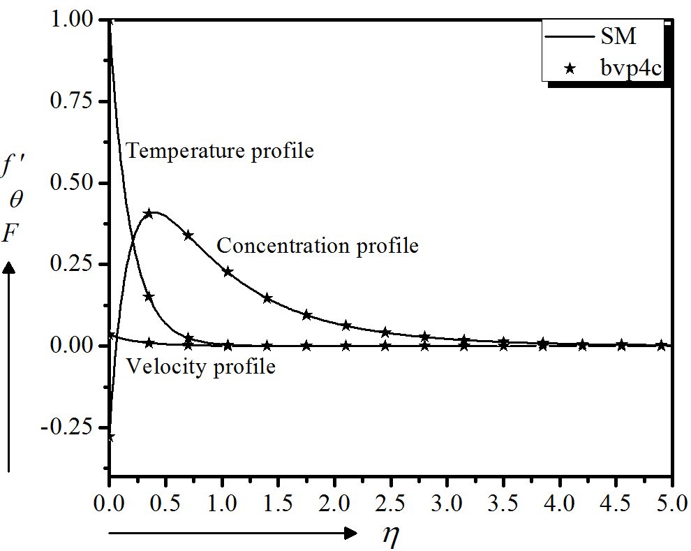
Equations (9)-(11) combined with the boundary conditions (12) are solved numerically using the Runge-Kutta method with the Nachtsheim-Swigert shooting technique (Nachtsheim and Swigert, 1965) for various values of the parameters nanoparticle volume fraction parameter $(\phi)$, Deborah number $(\beta)$, magnetic field parameter $(M)$, unsteadiness parameter $(A)$, slip parameter $(\delta)$, stretching parameter $(\gamma)$, suction parameter $(f_{w})$, electromagnetic field parameter $(\epsilon)$, Prandtl number $(Pr)$, Eckert number $(Ec)$, thermophoresis parameter $(Nt)$, Brownian motion parameter $(Nb)$, Lewis number $(Le)$ and chemical reaction parameter $(R)$. The step size is taken as $\eta=0.01$ and the tolerance criteria are set to $10^{−6}$. In order to strengthen the reliability of our results, a MATLAB boundary value problem solver called bvp4c is used. For numerical computations, [0, 5] is considered as the domain of the problem instead of $[0, \infty)$ as for $\eta \gt 5$ there is no noteworthy deviation in the results. The parametric values $\phi = 0.05$, $\beta = 0.5$, $M = 0.3$, $A = 0.3$, $\delta = 0.5$ and observed from Madhu et al., (2017) and Sithole et al., (2017) are set for Au-water nanofluid to verify the numerical results for both shooting method and MATLAB code showing in the Fig. 2.
Results And Discussion
Figure 2 is giving significant agreement to validate the numerical results attained by both shooting method and bvp4c function. But still for more contentment, it is necessary to certify our codes by comparing with some published articles of similar nature. For this purpose, we have analyzed the numerical values of local skin friction coefficient $f''(0)$ for the models investigated by several researchers. A remarkable agreement of these results with other models can be seen in Table 2.
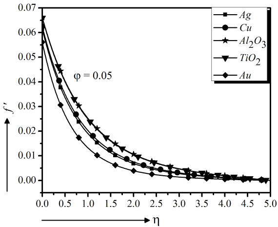
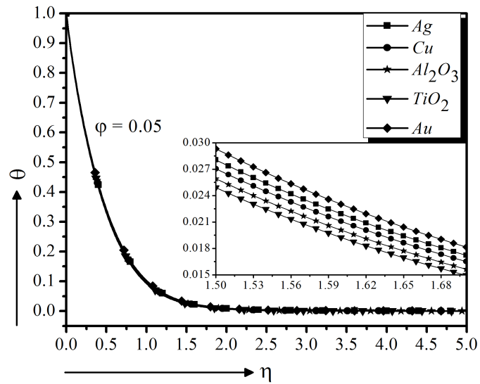
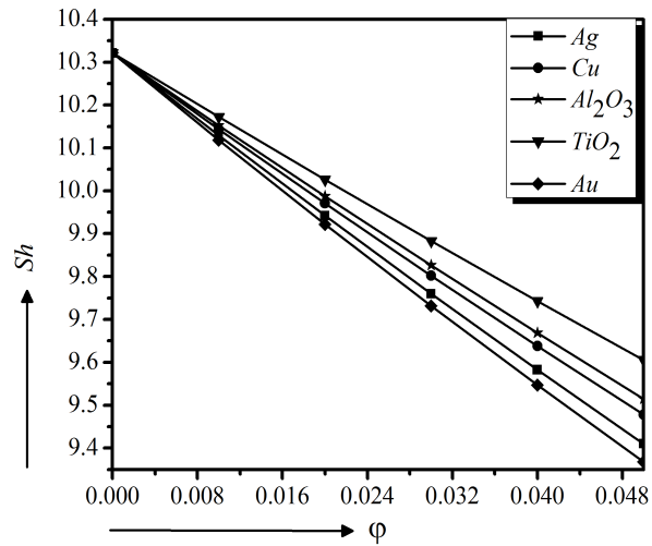
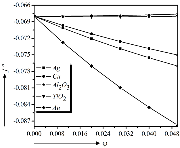
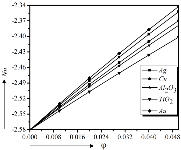
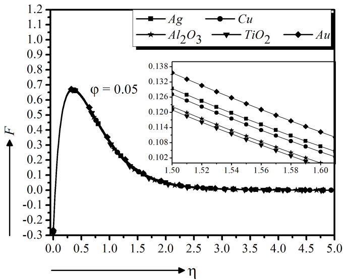
First, the numerical calculations of the velocity, temperature, concentration and heat transfer profiles are executed for water-based nanofluids using 5% volume fraction containing different solid nanoparticles $(Ag, Cu, Al_{2}O_{3}, TiO_{2}$ and $Au)$ one by one, in Fig. 3 to 8. It is observed in Fig. 3 that $Au - $water has lower velocity compare to other nanofluids $(Ag, Cu, Al_2O_3$ and $TiO_2 - \text{water})$ and it has higher temperature as well as is higher shown in Fig. 7. And friction (Fig. 6) and mass transfer (Fig. 8) rate are lower. As a higher heat transfer fluid with velocity control, $Au - $water nanofluid is chosen for the current model.
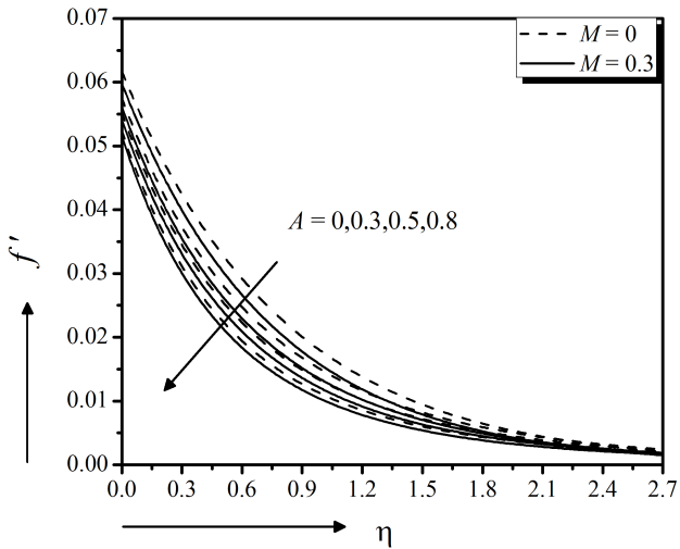
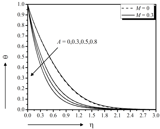
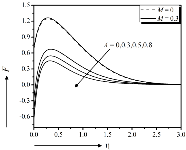
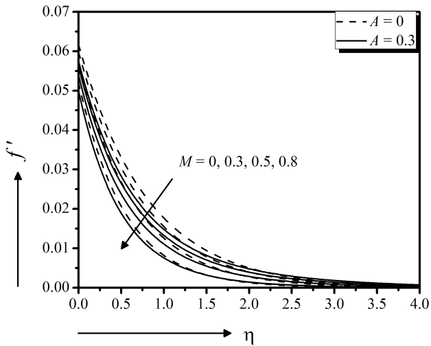
The unsteadiness parameter effect of the flow model on velocity, temperature, nanoparticle concentration field, local skin friction, Heat transfer and mass transfer coefficients are exposed in Fig. 9 to 14, respectively, both in the presence and absence of magnetic field effect. Figure 9 exerts the decreasing velocity $f'$ along the surface due to the raise of unsteadiness parameter A for both cases, $M = 0$ and $M = 0.3$. This indicates an associated reduction of the momentum boundary layer thickness near the surface and away from the surface. Simultaneously, it is also revealed that the magnetic field parameter $M$ produces a retarded force that slower the velocity of the flow. Furthermore, the steady case of the model is characterized by taking $A = 0$. It is observed from Fig. 10 that the temperature $ \theta $ decreases significantly with the increasing unsteadiness parameter and the magnetic field parameter effect is very negligible. This means that the less heat is transferred from the fluid to the surface and hence, the temperature decreases. It provides an important message that the cooling rate is faster for higher values of the unsteady parameter, whereas cooling may take longer during steady flows for both cases, $M = 0$ and $M = 0.3$. Figure 11 represents the declining effect of unsteadiness parameter $A$ on the solute distribution, both in the presence and absence of magnetic field effect. The mass transfer from the nanofluid to the surface is decelerated due to the increasing unsteadiness parameter $A$ which results lower concentrated fluid. The results are significantly similar to Madhu et al., (2017).
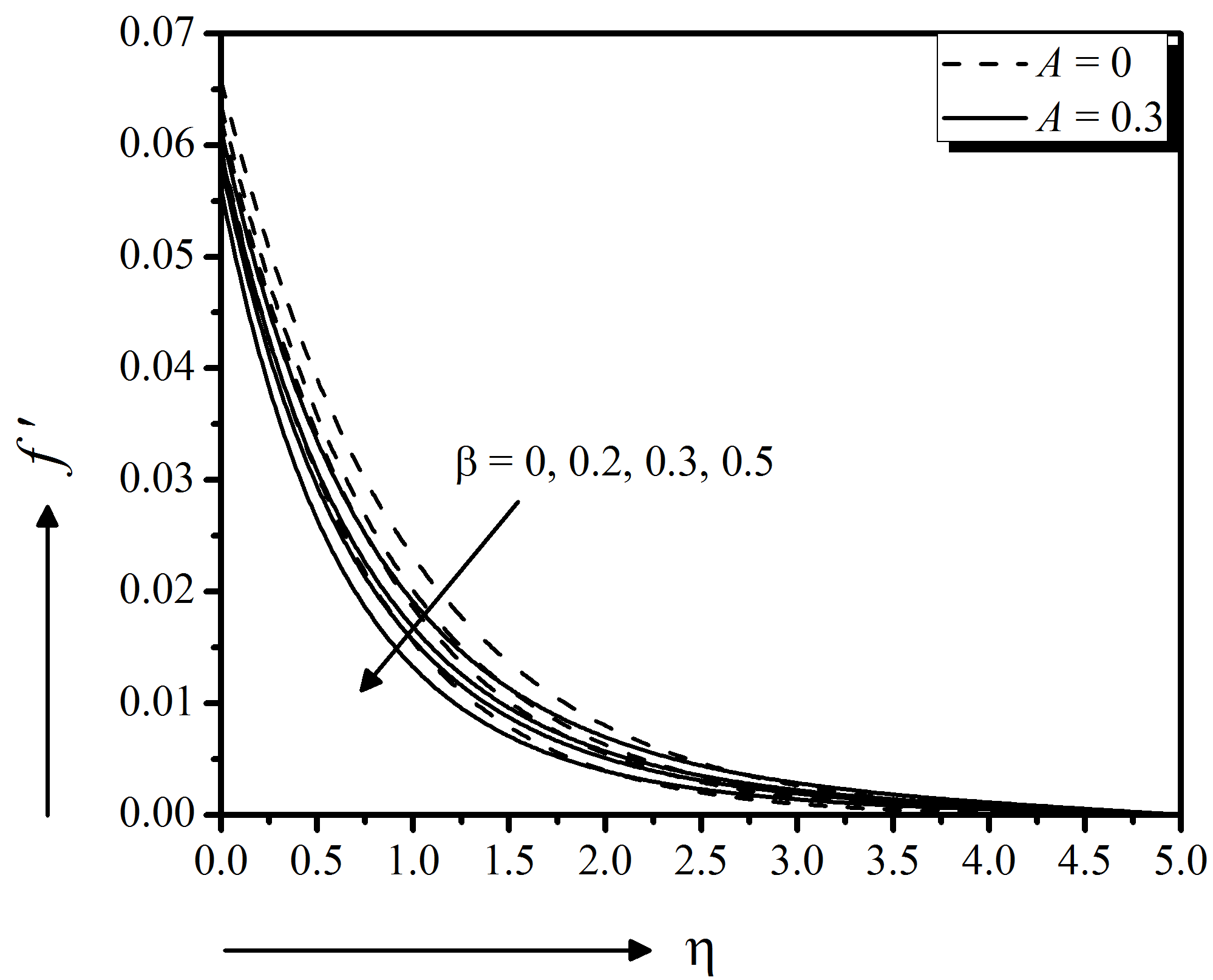
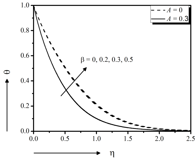
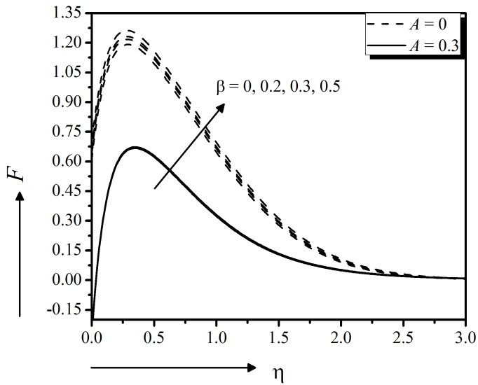
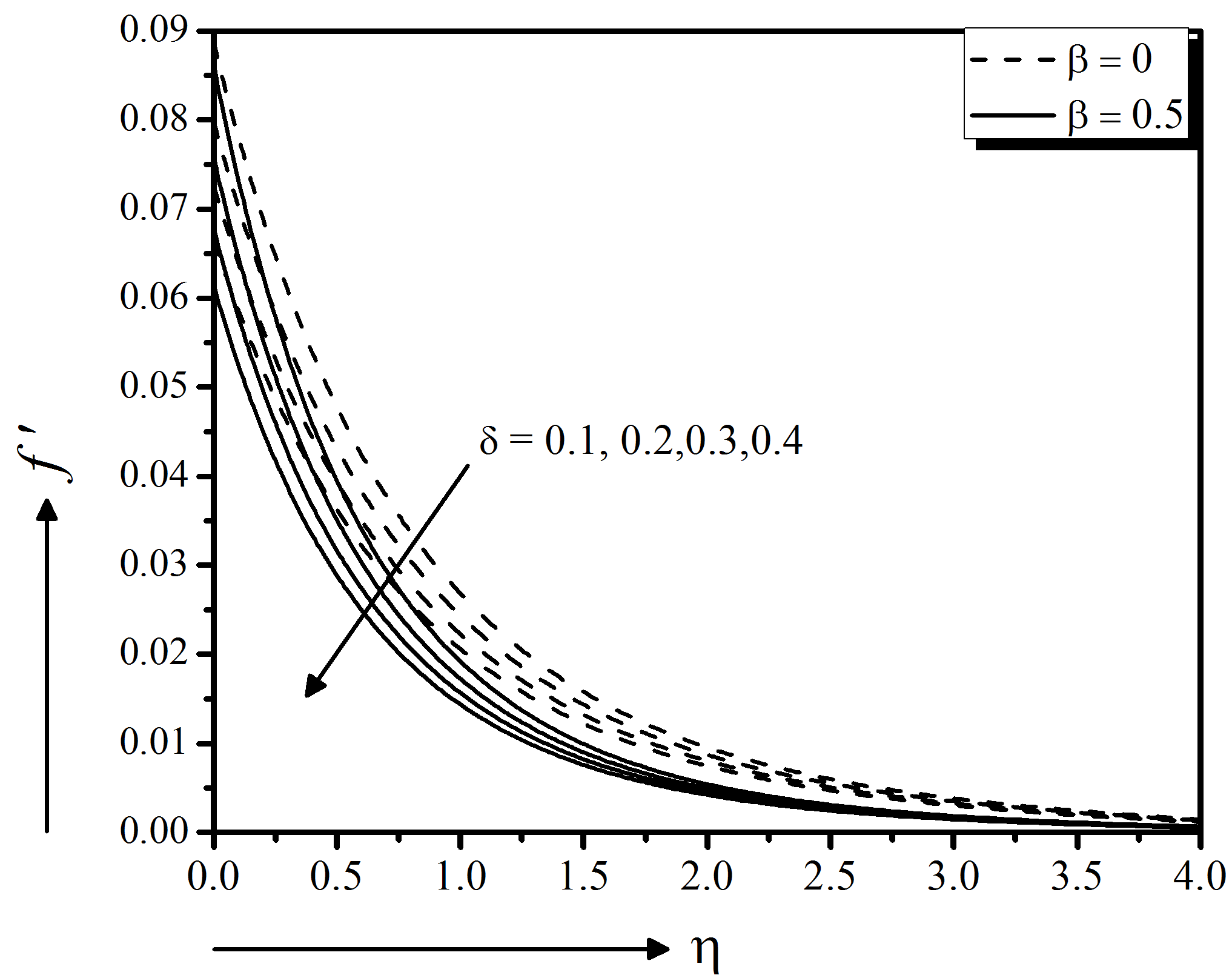
When the elastic stress is applied to the non-Newtonian fluid, the time during which the fluid achieves its stability is the relaxation time, which is greater for highly viscous fluids. The Deborah number $\beta$ deals with the fluid relaxation time to its characteristic time scale. Here $\beta = 0$ gives the result for Newtonian viscous incompressible fluid. The fluid with a small Deborah number exhibits liquid-like activities but large Deborah number communicates with solid-like materials able to conduct and retain heat better. Therefore, it is observed physically that gradually increasing the Deborah number can increase the fluid viscosity, which enhances resistance to flow and, as a result, the hydrodynamic boundary layer thickness reduces for Maxwell fluid, as shown in Fig. 12 for both steady $(A = 0)$ and $(A = 0.3)$ unsteady motion. These results are showing good agreement with Sadeghy et al. (2005). Figure 13 shows very negligible effect of the Deborah number on the thermal boundary layer for both cases $A = 0$ and $A = 0.3$. Thus, the heat transfer rate at the stretching surface increases with increasing $\beta$. From this analysis, it can be concluded that the elastic force endorses the heat transfer in Maxwell nanofluid. The higher values of $\beta$ on concentration are more pronounced for steady motion, in Fig. 14. Thus the mass transfer rate at the stretching surface decreases with increasing $\beta$.
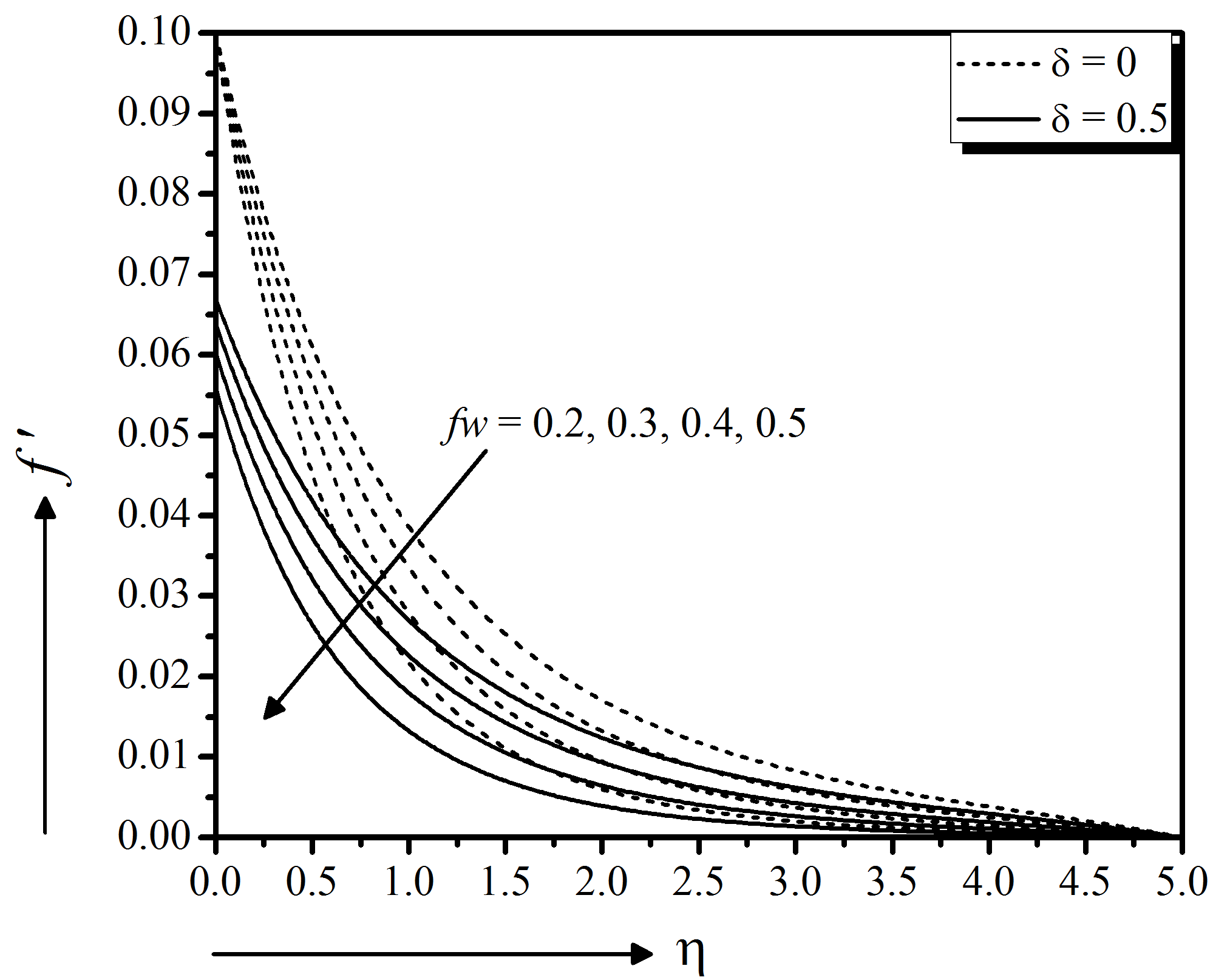
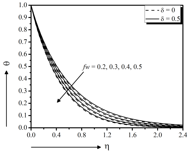
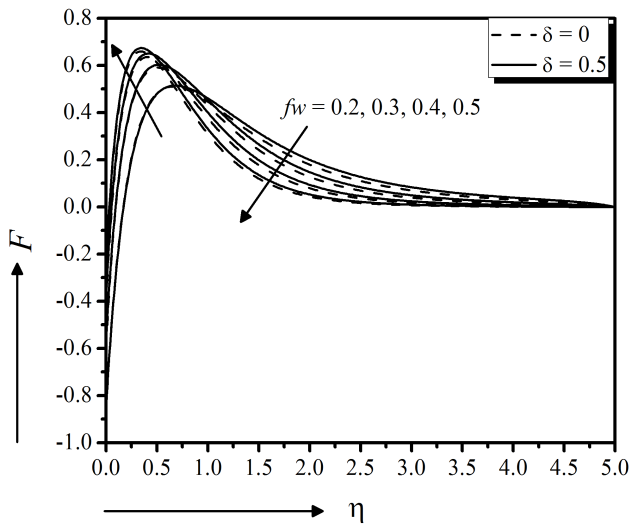
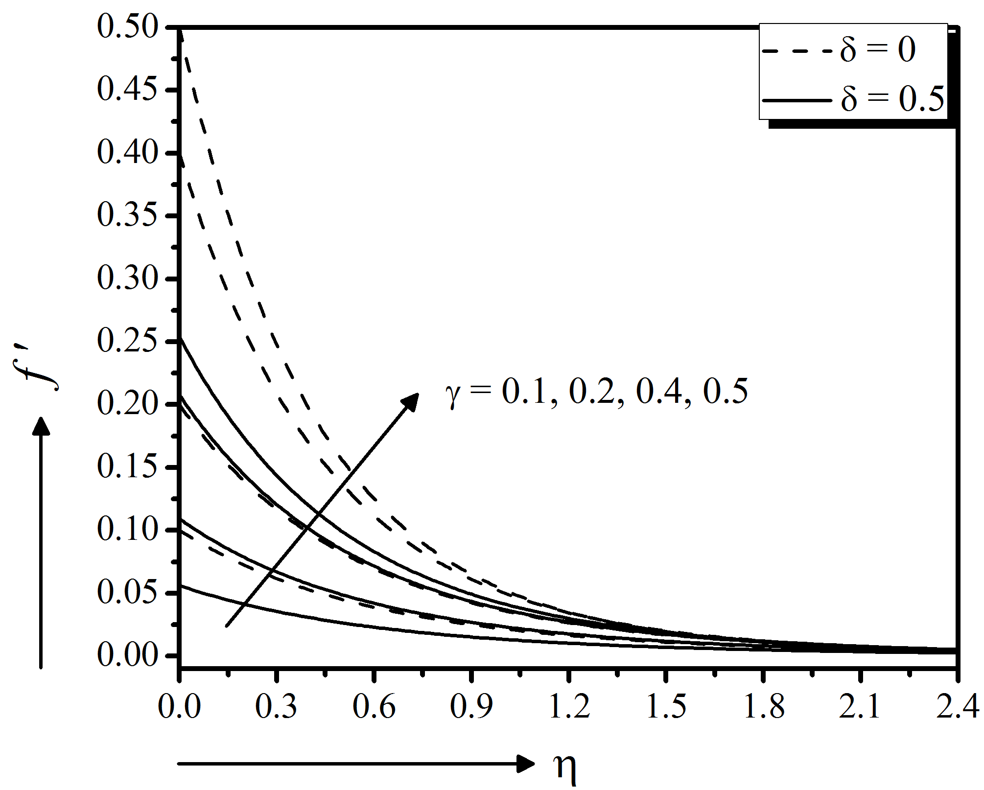
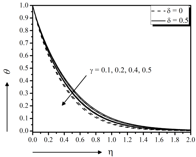
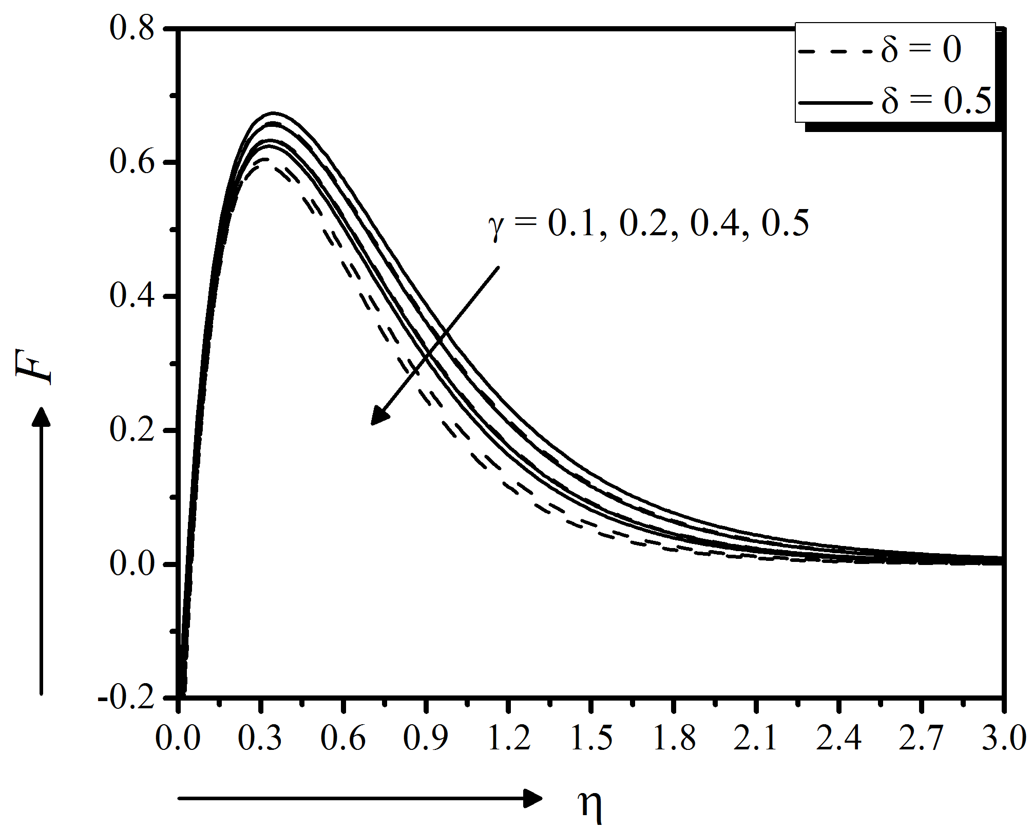
Figure 15 to 17 depict the suction effect on momentum, energy, and concentration distributions, respectively. From these figures it is clear that the momentum as well as energy distributions are decreasing function of suction showing good agreement with Nayak (2016) for both slip $(\delta = 0.5)$ and no slip $(\delta = 0)$ boundary surface. Physically, the imposed suction brings the distance of the fluid to the region closest to the surface by improving the viscosity which in turn decelerates the motion of the fluid. Moreover, the concentration profile increases near the surface but starts to decrease away from the surface with the higher suction. Moreover, an increase in stretching parameter $\gamma$ significantly enhances the flow velocity (magnitude) for both slip $(\delta = 0.5)$ and no slip $(\delta = 0)$ boundary surfaces, seen in Fig. 18. But the temperature and concentration profiles decrease with the increase of stretching parameter (Fig. 19 and 20).
The effects of magnetic field on momentum for both steady $(A = 0)$ and unsteady $(A = 0.3)$ cases are demonstrated in Fig. 21. It is observed that an increase in the magnetic parameter $M$ monotonically reduces the velocity profiles. This is the result of the effect of the magnetic field imposed on an electrically conductive fluid, which generates a drag force called Lorentz force against the flow direction along the surface to slow down velocity. In steady case, this situation is more significant. This is in accordance with the fact that the magnetic field is responsible for reducing the velocity of fluid flow. The current results in Fig. 22, similar to the findings carried out by Narayana and Gangadhar (2015), is that the velocity decreases as the slip parameter increase both in the presence and absence of the Deborah number.
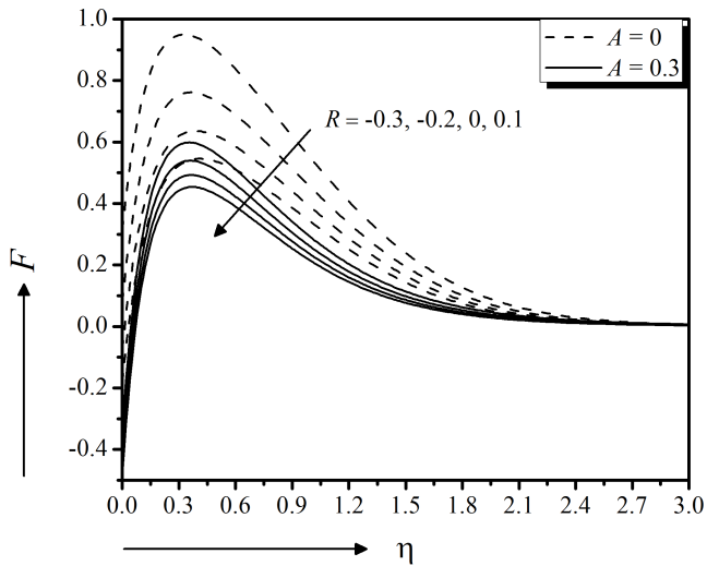
Figure 23 demonstrates the effects of chemical reaction on species diffusion for both steady $(A = 0)$ and unsteady $(A = 0.3)$ cases. It is exerted that higher destructive reaction rate parameter $(R \lt 0)$ enhances the concentration. However, concentration has opposite effects for generative chemical reaction parameter. The effect of chemical reaction parameter $(R \gt 0)$ is more outstanding in steady case. Physically, the larger values of destructive chemical reaction parameter deal with higher rate of destructive chemical reaction which deliberates the infected species more efficiently and hence the solutal distribution increases, Hayat et al., (2017). However, an opposite situation is observed for generative chemical reaction parameter.
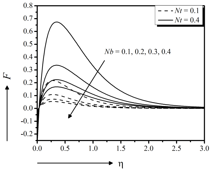
Figure 24 exposes the result in concentration in response to a variation in Brownian motion and thermophoresis parameters. It is found that the increasing values of the Brownian motion parameter cause the thickness of the concentration boundary layer to decrease (Sithole et al., 2017), that is, the concentration boundary layer thickness is larger with a lower Brownian diffusion. Therefore, the Brownian motion parameter $Nb$ facilitates diffusion of nanoparticles in the concentration boundary layer. Furthermore, the reverse environment is created by thermophoresis parameter $Nt$.
Finally, from the point of view of physical interest, the skin friction coefficient is useful to estimate the total frictional drag exerted on the surface. The Nusselt Number is used to characterize the heat flux from a heated solid surface to a fluid. The Sherwood number is used in mass-transfer operation. The effect of several variables on the skin fraction coefficient $(f'')$ the local Nusselt number $(-\theta')$ and the local Sherwood number $(-F')$ are arranged in the Table 3.
| Present work | ||||
|---|---|---|---|---|
| A | Madhu et al. (2017) | Sharidan et al. (2014) | bvp4c | SM |
| 0.8 | - 1.261211 | -1.261042 | - 1.261042 | - 1.261495 |
| 1.2 | - 1.377625 | - 1.377722 | - 1.377724 | - 1.377644 |
| A | $ \beta $ | $ \delta $ | $ \gamma $ | $f_{w}$ | $K_{cr}$ | $f''$ | $-\theta'$ | $-F'$ |
|---|---|---|---|---|---|---|---|---|
| 0.3 | 0.5 | 0.5 | 0.1 | 0.5 | -0.3 | -0.08776 | -2.34203 | 9.36811 |
| 0.5 | -0.09185 | -2.72907 | 10.9163 | |||||
| 0.3 | -0.08318 | -2.34671 | 9.38684 | |||||
| 0.3 | -0.10749 | -2.35676 | 9.42704 | |||||
| 0.4 | -0.38453 | -2.52075 | 10.08301 | |||||
| 0.3 | -0.07196 | -2.02166 | 8.08663 | |||||
| -0.2 | -0.08776 | -2.34300 | 9.37413 |
Conclusion
As a final point, the results obtained from the effects of various physical parametric effects on the characteristics of flow, heat and mass transfer are investigated and discussed extensively. The major outcomes drawn from the study of the present model can be summarized as follows:
- The heat transfer rate of Au-water is comparatively higher and the friction and mass transfer rates are lower.
- The friction rate is going lower for the increasing unsteadiness parameter, while the cooling rate and the mass transfer rate are much faster for higher unsteadiness parameter, whereas cooling may take longer during steady flows.
- The hydrodynamic boundary layer thickness is reduced for Maxwell fluid.
- Imposed suction can rule the momentum, energy and concentration distributions significantly.
- The magnetic field and slip velocity are liable for reducing the velocity of fluid flow.
- The concentration distributions are very much affected by chemical reaction and Brownian motion parameters.
Author Details
Department of Mechanical Eng., College of Engineering, University of Anbar, Ramadi, Anbar, Iraq
References
Rights and permissions
Open Access: This article is licensed under a Creative Commons Attribution 4.0 International License, which permits use, sharing, adaptation, distribution and reproduction in any medium or format, as long as you give appropriate credit to the original author(s) and the source, provide a link to the Creative Commons license, and indicate if changes were made. The images or other third-party material in this article are included in the article’s Creative Commons license, unless indicated otherwise in a credit line to the material. If material is not included in the article’s Creative Commons license and your intended use is not permitted by statutory regulation or exceeds the permitted use, you will need to obtain permission directly from the copyright holder. To view a copy of this license, visit http://creativecommons.org/licenses/by/4.0/
Cite this Article
DOI: http://doi.org/10.19026/rjaset.17.6031