Aarts, E. and J. Korst, 1989. Simulated Annealing and Boltzmann Machines: A Stochastic Approach to Combinatorial Optimization and Neural Computing. Wiley, New York, USA.
Research Journal of Applied Sciences, Engineering and Technology
A Novel Approach in Digital Controllers Design Using Metaheuristic Algorithms
Research Journal of Applied Sciences, Engineering and Technology 2020 17: 74-87
Cite This ArticleAbstract
Aim of this study is to present two optimal methods for adjusting parameters of PID controllers using Simulated Annealing (SA) and Particle Swarm Optimization (PSO) algorithms to achieve the desired goal intended for application of these controllers. Through adding intelligent techniques to the SA algorithm, it will lead to a higher speed and the reduction of the error in the PID controller. Available rules for setting PID parameters are commonly trial and error which involve various issues like being very time consuming, imprecise and facing a significant number of errors. Using performance measurement criteria and integrating them, an attainable method has been presented for setting these parameters which has a very high accuracy as wells as a significant speed, with a very low rate of error. Results obtained in this research demonstrate a considerable efficiency compared with that of other proposed methodologies.
Keywords:
Introduction
The proportional-integral-derivative (PID) controllers are among the most commonly used ones available in industry which meet various requirements of complex industrial parts. A variety of applications including networked control of a large pressurized heavy water reactor (PHWR) (Dasgupta et al., 2013), automatic voltage regulator (AVR) (Hasanien 2013; Kim et al., 2012),power plants (Glickman et al., 2004), Load Frequency Control (LFC) of power systems (Tan 2010), temperature controllers such as temperature controllers used in tunable semiconductor laser modules for optical communication systems (Wang and Yu 2012) or temperature controllers for a Polymerase Chain Reaction (PCR) (Dinca et al., 2009), compensation of a SVC load (Wang et al., 2008) and Variable-Speed Motor Drives (Shin and Park, 2012) can be named for these controllers, among others. Capability of these controllers in utilization in numerous applications is their great advantage. In addition, in conditions where the mathematical model of the process is unknown, usually these controllers are applied. Although, finding an efficient and optimal method of designing PID controllers which could be applied in variety of processes with a very low error rate, is highly challenging. Therefore, researchers continually work on finding the most optimal method for adjusting these controllers’ parameters. Methods used for setting these parameters can be divided into two general groups of classic and metaheuristic.
Approaches proposed by Ziegler and Nichols (1942) and Cohen and Coon (1953) are among experimental and classical ones, based on approximation. Fuzzy inference (Chang et al., 2009; Harinath and Mann, 2008), fuzzy simulated annealing (Ho et al., 2006), simulated annealing (Hung et al., 2008), Particle Swarm Optimization (PSO) (Gaing, 2004), genetic algorithm (Neath et al., 2014) and ant colony neural network (Cao et al., 2007) can be mentioned as metaheuristic techniques utilized for adjustment of PID controllers in literature.
Aim of this research is to provide an efficient optimal methodology that could be employed for all systems in most of processes and desired response could be obtained with a very low rate of error. In this study, to design and adjust a PID controller, two metaheuristic algorithms including Particle Swarm Optimization (PSO) and Developed Simulated Annealing (DSA) have been deployed. PSO algorithm is one of metaheuristic algorithms which deals with finding optimal response based on collective intelligence with inspiration from nature. Birds flying or fishes swimming in groups, are examples of this collective intelligence. Based on the desired search space, this algorithm has been used in both continuous and discrete fields (Kennedy and Eberhart, 1995; Vlachogiannis and Lee, 2006; Jin et al., 2007). Simulated annealing algorithm (SA) was first used in 1983 for optimization issues with Inspiration from solidification of molten metal (Kirkpatrick et al., 1983). First, an introduction on these two metaheuristic algorithms and then the way they are applied to obtain optimal responses would be discussed in herein. Moreover, some techniques will be presented in order to develop and increase the efficiency of these algorithms. General structure of PID controllers has been discussed accompanying with some explanations on application of PID digital controllers. A digital PID controller was adjusted using DSA and PSO algorithms and simulations of this controller have been presented for sample systems of Surface Mount Technology (SMT) and Automatic Voltage Regulator (AVR). Results obtained from simulations compared with that of other researchers demonstrated superior function of suggested strategies.
Materials And Methods
Artificial intelligence applied in scientific applications is an inspiration from natural intelligence showed by humans as well as animals. Many researchers have tried to present algorithms inspired from processes in nature, which could replace classical techniques in engineering applications that are based on complex mathematical analysis. Widely used fields of artificial intelligence applications include soft computing and optimization problems among others. Genetic Algorithm (GA) (Mashhadi et al., 2003), Ant Colony Optimization (ACO) (Dorigo et al., 1996), Tabu Search (TS) (Glover, 1990), Simulated Annealing (SA) (Vecchi and Kirkpatrick, 1983), Particle Swarm Algorithm (PSO) (Kennedy and Eberhart, 1995)and Neural Network (NN) (Tagliarini et al., 1991), can be cited among the most popular metaheuristic algorithms.
Standard SA algorithm: Simulated Annealing (SA) is the behavior of a molten metal in its cooling process and is considered as one of metaheuristic algorithms. In the molten metal, with the gradual decrease of temperature, the metal crystal forms a regular network and the final solid material will have the minimum level of energy. The idea of simulated annealing was first expressed by Metropolis et al. (1953). If one heats up a solid material and lets its temperature reach the melting point, then cools it down again, details of the result molecular structure will depend on the method and how it cools down. In gradual refrigeration for any given temperature, the probability of material particles having a certain level of energy is computed according to the Boltzmann distribution in statistical mechanics. This probability P, also called the transition probability is high at first and then decreases in proportion to temperature while the process progresses and is determined as per below relation:
$ P(\gamma) = exp(-\frac{\gamma\Delta f}{k_BT}) ~~~~~~~~~~~~~~~~~~~~~~~~ (1)$
Where $k_B$ is the Boltzmann’s constant, T is the temperature for controlling the annealing process and $∆E$ is change of the energy level. The simplest way to link $ΔE$ with the change of the objective function $Δf$ is to use $ΔE = γΔf$, where $γ$ is a real constant. For simplicity, one can use $k_B = 1$ and $γ = 1$. Thus, the probability P becomes (Yang, 2013):
$ P = exp(-\frac{\Delta E}{T}) ~~~~~~~~~~~~~~~~~~~~~~~~ (2)$
SA algorithm, by dominating local minimums would be able to find the absolute optimum answer. As well as approaching the better answer, this method accepts worse solutions, i.e., objective functions $(∆f > 0)$ with a non-zero probability in every repetition, unlike other common search methods.Provided the slop of temperature reduction curve is less than that of:
$ T = \frac{T_0}{1+log(K+1)} ~~~~~~~~~~~~~~~~~~~~~~~~ (3)$
SA algorithm will be convergent to the absolute minimum (Aarts and Korst, 1989), where $T_0$ is initial temperature, $T_k$ is temperature in each step and $k$ is step of iteration.
The current acceptance condition in SA technique is Metropolis criterion in which, provided the change rate of energy level be low, $∆E$ would be negative and “$exp(-∆E/T)$” would be bigger than 1 and hence the current mode would be accepted. However, if $∆E$ is positive, the probability of accepting this variation would depend on the amount of positive changes, temperature and the Boltzmann distribution function.
SA technique, which has its roots in Metropolis algorithm, first was presented by Kirkpatrick et al. (1983) for optimization purposes. Generating answers in the neighborhood of the current answer and calculating the effective variation in the objective function $(Δf)$ is the main idea in this method. In continuous problems, new variables are produced based on defining the neighborhood radius and the previous variable. In the production of new variables, random movement in the search space will be limited by a radius called neighborhood radius. This radius is decreased simultaneous with the temperature reduction and controls the variation range of variables. The best answer has been obtained, provided the new answer is definitely accepted. Otherwise the new answer would be accepted considering a probability and hence the movement would be towards increase of the objective function. In SA algorithm, movement capability of network elements in the space between molecules is determined by temperature. As search process goes on, temperature decreases in a specific manner. Actually, in every repetition of the algorithm it is the system temperature that determines the acceptable subspace to be searched. Almost all of produced answers will be accepted regardless of the objective function value in high temperatures. On the other hand, inappropriate answers have a less chance of acceptance, as the algorithm progresses and temperature decreases. Actually, in any temperature, the acceptance probability of an answer depends on the increase amount of the cost function. If the slope of the temperature reduction curve is not small enough, crystal network of the metal faces an immediate cooling-off which in turn would result in an erratic crystal structure that could not have the minimum energy level. To increase search opportunity in algorithms where temperature reduction rate is more than the marginal rate, algorithm repetition in the temperature reduction process has been considered for every stage and the numbers of this repetition is called Markov chain length.
Developed SA (DSA) algorithm: Initial temperature is a crucial factor in SA approach which can affect rate and convergence of the algorithm. In Yip and Pao (1995), the simplest method, i.e., choosing a constant amount for the initial temperature, has been used for determining the initial temperature. In this research, initial temperature at the beginning of the algorithm, based on the γ which is indicative of probability of the accepted modes through Boltzmann probability function (Pao et al., 1999), has been determined in proportion to the PID parameters. When $γ$ equals to 20%, it implies there is a chance of 20 percent acceptance for all states. The new variable that is generated in the initial temperature will be produced similar to its generation during the main algorithm. This monitoring tactic for determining the initial temperature has more efficiency compared to variable random production method for determination of a specific number of accepted states. In this study, percentages from 10% to 90% have been examined which revealed 20% is the optimal percentage for $γ$. In addition to maintaining accuracy in the convergence of the algorithm, this percentage will have a higher speed compared to other values for determining the initial temperature.
Dynamic Definition of Markov Chanin: Another characteristic that determines the cooling schedule is length of Markov chain. Provided this length is too short it will result in losing the opportunity. On the other hand, if it is too long, optimization time increases considerably. This value and its importance have not been discussed enough in literature and often is considered as a constant value. In Kirkpatrick et al. (1983), while defining the cooling function, the following relation has been considered:
$ T_k = \alpha T_{k-1},\ \alpha = 0.9 ~~~~~~~~~~~~~~~~~~~~~~~~ (4)$
Number of iterations in internal loop in proposed algorithm herein is considered in a way that number of attempts for each temperature in average is equivalent to 10 acceptances per each internal loop, provided that the total number of efforts do not exceed 100 times the number of internal loop iterations. Pao et al. (1999) in their research study suggested that number of iterations in internal loop is dependent to the problem and recommended constant values 5000 and 20000 as Markov chain length. Sohn (1995) expressed that the number of iterations in internal loop is fixed but related to the problem. Wong and Constantinides (1996) for TSP problem, proposed the number of iterations per each temperature to be equal to the square of the number of cities. Wu and Chow (2007) has considered the number of iterations in constant temperature for continuous test functions as a fixed amount that can be selected in a range of 10 to 4000. The number of iterations in a temperature for the SA and Self-organizing and Self-evolving Neurons (SOSENs) is set to five for all the TSP problems (Wu and Chow, 2007). Lin et al. (1993) is one of few researches in which using an integrated Simulated Annealing (SA) and Genetic Algorithm (GA) methodology called AG, a variable length for Markov chain has been considered. In Lin et al. (1993), length of Markov chain was assumed according to the population size in GA algorithm and in each step, proportionate to the equilibrium conditions of SA algorithm. Then it was calculated and put in search process as different values. He (2002) in a combined approach, designed by neural network, has used an iteration number at any fixed temperature which is proportional to the production, evaluation and updating all neurons according to the Metropolis criterion.
In this study, a particular perspective on the number of iterations at each temperature is proposed. Indeed, increased length of Markov chain provides a sufficient opportunity for search algorithm at a specific temperature, that is so close to the optimal point as much as possible. For optimum use of appropriate temperature, chain’s length can be revised to obtain the optimal value according to the temperature at which the search takes place. While having a defined fixed number of iterations in the search loop at constant temperature conditions, Markov chain’s length reflects the same need for having an equal effort at different temperatures for the search algorithm that does not seem logical. SA algorithm, to achieve an optimal solution, requires an effort that is proportionate to the temperature of search process, as it is possible to be close to the optimal energy point more quickly at a certain temperature. In other words, the Markov chain’s length must be defined differently for each working temperature. Accordingly, in the proposed algorithm in this study, the number of iterations at a temperature, instead of being defined as proportional to the number of iterations in the inner loop, has been taken proportional to the number of acceptances happened in the inner loop. Number of desired acceptances can be reduced during implementation of the algorithm linearly according to the temperature decline. With linear decline of the maximum acceptance in Markov chain which is indicative of chain’s length, again in practice, the number of iterations increases in the effective interval of search process and commensurate with temperature decrease. Certainly, it is expected that the number of acceptances decreases according to the temperature reduction while approaching toward freezing point, or in other word, creation of the low-energy crystalline forms. In fact, the Markov chain’s length to suit what is happening at any temperature, has found a dynamic definition, so that at the middle temperature, interval (mushy state temperature) becomes longer and searching opportunity increases in this interval.
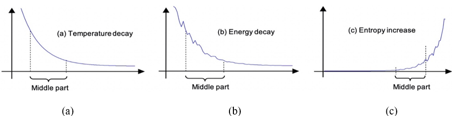
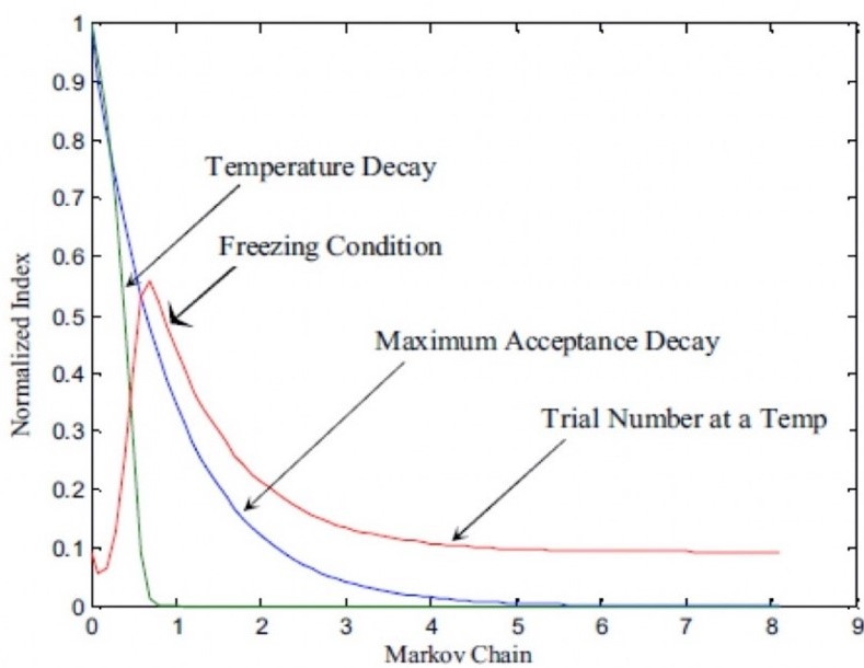
Proper value of linear reduction factor for maximum acceptance in Markov chain, regarding comparative studies, has been considered as 0.9, in this research. Fig. 1, for instance, demonstrates that temperature decreases through an exponential curve that can be divided into three different intervals. The First interval that is the initial part of the curve indicates a very high temperature state and it should be passed with a steep slope. The second interval is the middle part of the curve in which the gradient decreases and is considered as the effective range of the algorithm's performance. Finally, the third interval is the final part that provides the conditions of convergence and also helps achieve optimal energy at a low temperature. In this interval, changes of temperature occur with a low slope. The Algorithm proposed in this study emphasizes on an effective range in optimal performance of search algorithm that is the middle interval. Therefore, by dynamic definition of the Markov chain’s length, search operations in the algorithm are improved and hence in the middle part there would be more effort. As shown in Fig. 2, with reduction of temperature from its initial value, the number of required efforts for successful search in a Markov chain increases. Obviously, this increase in the middle range of temperature would be appropriate. However, according to a new and dynamic definition of Markov chain, after passing the effective temperature, due to dramatic declines in the maximum number of acceptances in a Markov chain and to reach a gentle gradient of temperature, the number of attempts required to achieve the maximum desired acceptance will be reduced intensively. This approach provides a proper distribution of iterations in the search process, in which the amount of algorithm's effort will be distributed according to the interval of activity. As a result, this algorithm increases the number of iterations for optimal search in the middle part and modifies the fixed definition of Markov chain’s length through decreased effort at the initiation as well as final temperature range and increases the middle range.
In this study, Markov chain’s length has been taken equal to 20 times of γ, which has been determined at the beginning of the search process and will be reduced during the algorithm with a 95% coefficient. This kind of definition for the Markov chain not only improves the convergence rate substantially, but also enhances accuracy of the algorithm by the optimal distribution of the number of efforts in the search process. In this study, the convergence condition of the algorithm or the freezing temperature has been considered as the state in which the minimum and the maximum energy in the Markov chain’s length would be equal to three decimal places.
Particle Swarm Optimization (PSO)
Particle Swarm Optimization (PSO) algorithm, as a novel method by an inspiration from birds flying or fish swimming in groups to search for food, aims to find the optimal answer. At the beginning, the particles are scattered in the search space randomly and that is how this algorithm works basically. Every particle in the search space is an agent to find a possible answer and all particles approach the optimal answer as time goes on, while they will benefit not only from their own search results, but also from that of the group. An efficient and effective search by the group of particles in the search space is the goal in this algorithm. Particles approach to the best and most suitable answer. The change of each particle’s position will be calculated by the cinematic equations while each particle’s velocity is considered constant in this algorithm. The particle’s velocity is affected by its velocity in the prior moment, particle’s deviation amount from its best position ever obtained and the distance from the best position ever obtained by the whole group. This algorithm was first applied by Kennedy and Eberhart (1995). N particles move in a D dimensional search space in this algorithm. Every Particle modifies its movement using its own and other particles’ experience and regulates its position in order to approach the best answer. The position of the ith particle in the D dimensional space and its velocity are determined with the Xi=(xi1,xi2,…,xiD) and Vi=(vi1,vi2,…,viD) vectors, respectively. While particles are moving in the search space, every particle calculates the required velocity vector for the next stage to move towards the optimal position by comparing its best position ever obtained to its current position while considering the best position ever obtained in the whole group of particles. Personal best (Pbest) is the best position the ith particle has reached so far and is presented as below:
$ Pbest_i = (Pbest_{i1},\ Pbest_{i2},\ ...,\ Pbest_{iD}) ~~~~~~~~~~~~~~~~~~~~~~~~ (5)$
Also, the position of the best answer obtained by the whole group is determined by global best (Gbest) as follows:
$ Gbest = (Gbest_1,\ Gbest_2,\ ...,\ Gbest_D) ~~~~~~~~~~~~~~~~~~~~~~~~ (6)$
Therefore, the ith particle’s velocity for the new movement is calculated by equation (7), which depends on its velocity in the prior step, its own experience and the orientation towards the best answer in the group:
$ V_i^{(K+1)} = C_0V_i^{(K)} + C_1.rand(Pbest_i - X_i^{(k)}) + C_2.rand(Gbest - X_i^{(k)}) ~~~~~~~~~~~~~~ (7)$
The constants C1 and C2 determine the particle’s own effect and the effect of collective intelligence on velocity, respectively. These constants are known as acceleration or cognition coefficientsand determine how the effective factors influence the velocity production and have been determined in some research works in a way that at the beginning of the algorithm the particle’s own effect overcomes that of the group and as the search process progresses, the collective intelligence will have more effect on the particle’s orientation (Franken and Engelbrecht, 2005; Seo et al., 2006).
In this study C1 and C2 have been chosen as 2 and 0, respectively at the beginning of the algorithm. But as the search process continues, C1 decreases while C2 increases, both linearly and finally reach amounts of 0 and 2, respectively. The C0 constant which is for the impact of the prior moment’s velocity on the current velocity, is set to 1 at the beginning of the algorithm and linearly falls to 0 at the end of the search process. Considering the current velocity vector and the prior position, the particle moves towards the destination according to the following equation:
$ X_i^{(k+1)} = V_i^{(K+1)} + X_i^{(k)} ~~~~~~~~~~~~~~~~~~~~~~~~~~ (8)$
Considering equations (7) and (8), it can be seen that the particles’ movement in the search space can be possible with the aid of a suitable definition of velocity as the controlling parameter in this algorithm. As it can be seen, the particles’ velocity in the PSO algorithm determines the orientation towards the optimal position in every step.
Digital and Analog PID Controllers: PID controllers are among the most practical as well as industrial controllers. These controllers operate based on three proportional, integral and derivative control actions. The proportional operator multiplies the error signal by a suitable gain and provides the controller’s output. The integral and derivative operators, conduct the integration and derivation on the error signal respectively and provide separate output for the controller. Thus, in the PID controller, a triple control command is generated as follows:
$ u(t) = K_pe(t) + K_i \int e(t)dt + K_d\frac {de(t)}{dt} ~~~~~~~~~~~~~~~~~~~~~~~~~~ (9)$
in which Kp, Ki and Kd are the proportional, integral and derivative coefficients, respectively.
Basic features of PID controllers, including reduction of costs and high speed in processing digital systems, among others, make them substantially valuable. Therefore, a digital PID controller has been utilized in this study to employ the optimal proposed method by two metaheuristic algorithms.
The digital form of this controller in the time domain is as below (Ogata, 2002):
$ U(t) = K_pe(t) + K_i \sum_{j=0}^k e(j)T + K_d\frac {e(k)-e(k-1)}{T} ~~~~~~~~~~~~~~~~~~~~~~~~~~ (10)$
Zero Order Hold and the Nyquist theorem: In order to use the digital PID controller in analogue industrial processes, it is required to use a conservator and a sampler (Ogata, 1995), so that the digital signal related to the output of the PID controller can enter the system while on the other hand a digital input is provided for the PID controller. In this study, a zero-order conservator and a sampler have been utilized. In addition, the Nyquist theorem (Oppenheim et al., 1996) should be considered and hence the sampling frequency must be more than twice of the highest frequency in the system so the system does not get in trouble while sampling in the closed loop.
Performance Criteria: To measure the performance of a PID controller, there have been some criteria defined as equations (11)-(14) (Oviedo et al., 2006), namely, integrated absolute error (IAE), integrated of time-weighted-absolute-error (ITAE), integral of squared-error (ISE) and integrated of time-weighted-squared-error (ITSE):
$ IAE = \int_0^T |e| dt ~~~~~~~~~~~~~~~~~~~~~~~~~~ (11)$
$ ITAE = \int_0^T t|e| dt ~~~~~~~~~~~~~~~~~~~~~~~~~~ (12)$
$ ISE = \int_0^T e^2 dt ~~~~~~~~~~~~~~~~~~~~~~~~~~ (13)$
$ ITSE = \int_0^T te^2 dt ~~~~~~~~~~~~~~~~~~~~~~~~~~ (14)$
In this study, percent of overshoot and above-mentioned parameters have been considered either separately or collectively when the cost function hits the minimum, to optimize performance of PID controller using metaheuristic algorithms.
Proposed Method
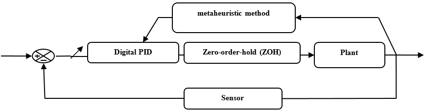
In this study, a digital PID controller with a zero-order hold has been employed. Regarding explanations presented for two metaheuristic algorithms, i.e., SA and PSO, the process is as Fig. 3. As it can be seen in this figure, with the input of the system which is a unit step function, the output is produced every instance and based on that, the metaheuristic algorithm, using performance criteria as the objective function, searches for the PID controller’s coefficients to reach the optimal response.
Proposed PSO-PID Controller:
- Step 1: Determine the number of particles and acceleration coefficients
- Step 2: Random determination of initial position and particles’ cost function
- Step 3: Determine vector of best position obtained by every particle (Pbest)
- Step 4: Determine the best position obtained by all particles (Gbest)
- Step 5: Determine particles’ new velocity vector based on Eq. (7)
- Step 6: Determine particles’ new position based on Eq. (8)
- Step 7: Check the condition for stopping the search process and continue the algorithm from Step 3, if it has not been satisfied
Proposed SA-PID Controller: SA algorithm has been applied with techniques proposed above to adjust the PID controller, while design of this controller is based on the following stages:
- Step 1: Determine optimal initial temperature according to the algorithm’s main loop variable production mechanism and equal to 20% acceptance and 100 times number of internal loop iterations.
- Step 2: Randomly determine the problem’s input variables (PID controller’s parameters) and define the initial amount of the neighborhood radius and reduction coefficient of neighborhood radius.
- Step 3: Determine the Markov chain’s length dynamically, proportional to the number of acceptances occurred and equivalent to the initial temperature’s acceptance coefficient for the number of iterations of the inner loop.
- Step 4: Determine the new variables around the previous accepted variables, proportionate to the neighborhood radius.
- Step 5: Determine the new variable’s cost function.
- Step 6: Check the Metropolis acceptance condition and determine the current variables.
- Step 7: Determine the minimum and the maximum of the inner loop and determine the amount and the vector of the outer loop’s minimum variables.
- Step 8: Go to Step 4 if the inner loop’s iteration has not come to an end yet, proportionate to the Markov chain’s dynamic definition in Step 3.
- Step 9: Reduce the Markov chain’s length (number of acceptances required for the inner loop’s iteration) by 90%.
- Step 10: Determine the new temperature based on the temperature reduction function, “ $T_{k+1} = T_k/(1+log(k))$ ”, which k = Outer Loop Counter.
- Step 11: Check the equality of the minimum and the maximum of the cost function to three decimal points in the inner loop search process, as the algorithm’s convergence condition and continue the algorithm from Step 4, if the convergence condition has not been met.
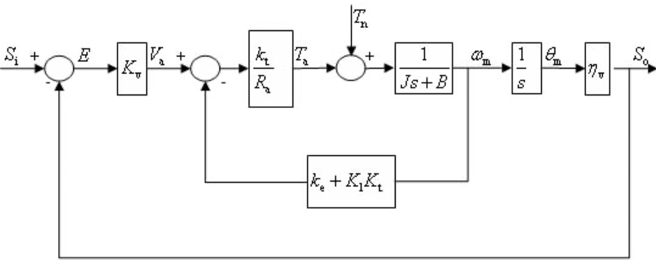
SMT Motion System: The purpose of Surface Mount Technology (SMT) system is to move the head of instruments from one point to another. This system has been modeled differently in literature. This system contains a servo driver with a motor. In Du (2004), a model for the multi axis SMT motion system has been presented. The block diagram of a motion system with disturbance is presented in Fig. 4.
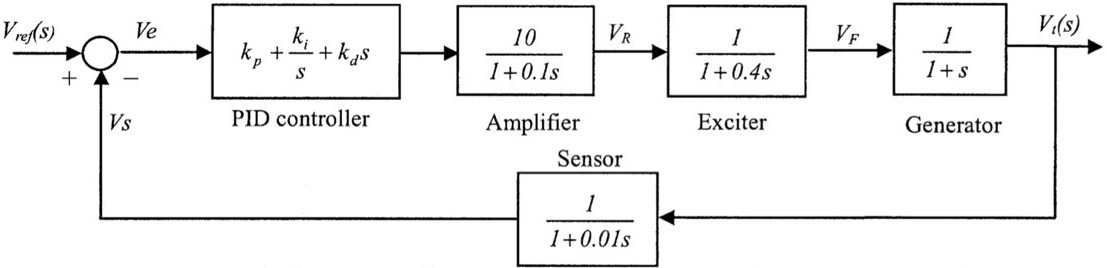
Automatic Voltage Regulator (AVR): The voltage of synchronic generators’ terminals can vary, provided the nature of the load changes. Thus, maintaining the voltage in a specific range is desirable. In order to fix the synchronic generator’s terminal voltage with different loads, the automatic voltage regulator (AVR) is applied. A simple block diagram of this system is shown in Fig. 5.
This system has four main parts including an amplifier, a driver/exciter, a generator and a sensor. To control this system, a PID controller adjusted by two proposed methods in this study has been applied and simulation results thereof have been presented below.
Result And Discussion
Simulation of PSO-PID and DSA-PID controllers for SMT: To simulate a digital PID controller and optimally adjust it using PSO and DSA algorithms and search for the best coefficients for the controller, an SMT motion process (Yachen et al., 2007) has been applied herein as the controlled system.
SMT’s transform functions for X and Y axes are as follows:
$ G_X(S) = \frac {46.78} {0.001926 S^2 + 0.1549 S} ~~~~~~~~~~~~~~~~~~~~~~~~~~ (15)$
$ G_Y(S) = \frac {78.23} {0.002651 S^2 + 0.2486 S} ~~~~~~~~~~~~~~~~~~~~~~~~~~ (16)$
A constant disturbance torque of TL=2 has been taken in this process. It should be stated that the SMT system does not limit the proposed method in this study and the given steps for SA and PSO approaches are independent from the kind of process. Simulation and optimization of SMT process has been performed in MATLAB 7.0 software while using a computer with 2GHZ of CPU and 512Mb of RAM. Results presented in Yachen et al. (2007) are for a digital controller which is used for obtaining the minimum amount of ITAE in the SMT motion process which has been designed by the common SA algorithm. In this study, PSO and DSA algorithms have been deployed. To compare results obtained by these two proposed algorithms in this study with that of presented by Yachen et al. (2007), the same approach in the objective function and the controlled process has been considered. Simulation results have been given in Table 1.
To complete simulation and present the proposed algorithm’s capabilities in optimization of the PID controller, different objective functions have been considered separately or in a combination with the percent of overshoot. Results are for 20 runs for every objective function and the best, worst and the average have been presented in Table 1 and 2.
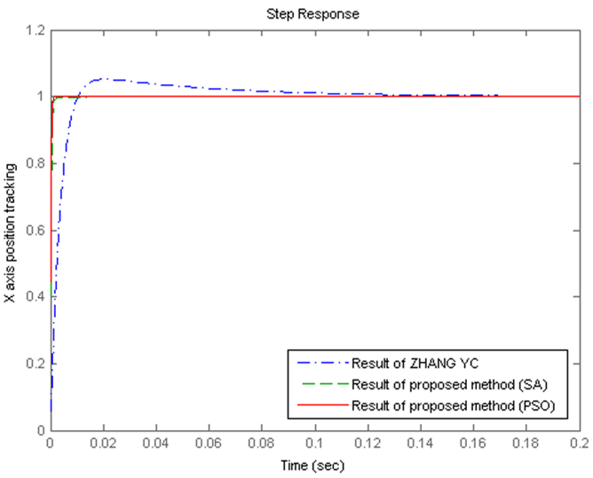
As it can be seen in Table 1, for the ITAE for X axis, the minimum amount of 3.24E-7 with PSO and 9.27E-7 with DSA have been acquired, respectively. While the result presented by Yachen et al. (2007) is 1.91E-5, which demonstrates results obtained in this research using both proposed methods are well better than that of Yachen et al.(2007). Of course, according to Table 2, overshoot for SA-PID controller is 0.930 and for PSO-PID controller is 0.423 which are well better than the overshoot of the controller in Yachen et al. (2007). Actually, by maintaining the overshoot in a desirable as well as a reasonable range, a very lower amount of error and ITAE have been obtained. The system’s output step response is presented in Fig. 6.
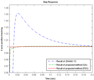
As it is obvious from Fig. 6, results of proposed methods in this study are very close to each other and are almost the unit step. But results of Yachen et al. (2007) are very different from the unit step and because of this difference between the reference input and the output, they show a higher error rate and therefore higher ITAE. Figure 7 shows Fig. 6 in a zoomed-in state, so the percent of overshoot resulted from proposed methods can be compared with that of Yachen et al. (2007).
According to Table 1, for the ITAE for Y axis, minimum amounts of 7.7E-7 and 5.37E-7 have been obtained by PSO-PID and DSA-PID controllers, respectively. While Yachen et al. (2007) has gained the minimum amount of 3.40E-6 for ITAE for Y axis. Figure 6 shows response of controlled SMT process for Y axis.
As illustrated in Fig. 8, system’s responses with PSO-PID and DSA-PID controllers, have reached the unit step very fast with pinpoint accuracy and low and reasonable overshoots which are 0.9886 and 0.6062 for DSA-PID and PSO-PID controllers, respectively, in contrast to that of presented by Yachen et al. (2007), that shows a considerable deviation from the unit step and a slow convergence to the final amount.
Simulation of PSO-PID and DSA-PID Controllers for AVR System: Herein, digital PID controller adjusted by PSO and DSA approaches has been employed to simulate the Automatic Voltage Regulator (AVR) system (Gaing, 2004) and the goal is to adjust it as desired. Gaing (2004) has considered a criterion using the rise time, settling time, percent of overshoot and the steady-state error as per equation (17) and the goal is to minimize or maximize it as a performance criterion:
$ W = (1-e^{-\beta}) (M_p + E_{ss}) + e^{-\beta} (t_s - t_r) ~~~~~~~~~~~~~~~~~~~~~~~~~~ (17)$
Which β is the weighting factor, Mp is the overshoot, tr is the rise time, ts is the settling time, Ess is the steady-state error and e is the error.
Considering this criterion for the proposed algorithms, unsuitable fluctuating dampedresponses can be found. Therefore, by taking this assessment criterion into account, the stability of the system has to be checked using Routh-Hurwitz criterion. Some parts of the response with amounts more or less than 1 that are located in the middle time range will be obtained by this criterion which are actually local minimums or maximums of the response in different periods and for removing these undesired responses a compound assessment criterion should be used. In this study, the assessment criterion of Gaing (2004) along with the Integrated of Time-weighted-Absolute-Error (ITAE) have been utilized as the compound assessment function to reach the minimum. In this case, responses that have unsuitable status in the middle time range, cannot be regarded desirable due to high ITAE and hence are not accepted as answers of the problem. Simulation results of the digital PID controller using both proposed methods compared to that of Gaing (2004) are presented in Table 2.
Gaing (2004) has gained 1.71 and 7.48 as overshoots for ß=1 and ß=1.5, respectively. According to Table 2, corresponding overshoots using PSO-PID controller are 0 and 0.423, respectively, with reasonable amounts of ITAE, which demonstrates a substantial improvement.
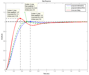
Amounts of the assessment function obtained in this study which was set to reach the maximum amount considered by Gaing (2004), for ß=1, have reached 12.72 and 11.75 using DSA-PID and PSO-PID controllers, respectively. In other words, the proposed techniques have produced very much desirable answers to increase the assessment function. According to Table 2, these responses have been obtained while, ts and tr are both reasonable. Figure 9, illustrates the step response obtained by both proposed approaches compared to that of Gaing (2004), for β=1.
As it is apparent from Fig. 9, results obtained by PSO-PID and DSA-PID have very lower overshoots and ITAE total errors without any undershoots and have reached desirable amount of 1, very fast.
As per Table 2, overshoots for both amounts of β, i.e., 1 and 1.5, are 0.025 and 0.930, respectively for DSA-PID controller. Obtained results show a significant improvement in terms of a considerable reduction of overshoots, compared to results presented in Gaing (2004).
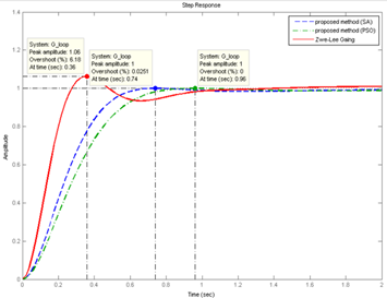
Figure 10 depicts step responses generated by DSA-PID and PSO-PID, in comparison with that of Gaing (2004) for β =1.5, in which overshoot has fallen very much in this case and the response has a very lower error rate and has converged the adjusted amount faster.
When β is 1.5, ITAE is 3.991 and 3.842 for PSO-PIDD and DSA-PID respectively, which proves a major improvement in comparison with results presented in Gaing (2004). Responses of proposed techniques have reasonable settling time (ts) and rise time (tr) and their overshoots decline substantially with very lower undershoots. The assessment function (W) while β is 1.5, has reached amounts of 4.156 and 3.126 for DSA-PID and PSO-PID, respectively which shows a significant increase comparing to that of Gaing (2004). Thus, proposed methods for the AVR system with the purpose of fixing the response on a specific level, have been able to obtain results which have lower amounts for total error and overshoot and hence are more desirable.
| Result of proposed method | |||||
|---|---|---|---|---|---|
| Plant | PSO | SA | Yachen et al. (2007) | ||
| X axis | PID Controller coefficient | Kp | 13.04 | 8.43 | 1.16 |
| Ki | 1.28 | 2.82 | 15.66 | ||
| Kd | 0.013 | 0.015 | 0.01 | ||
| Overshoot (%) | Min | 0 | 0 | 0.19 | |
| Max | 0.2531 | 0.1486 | 8.7 | ||
| Mean | 0.1031 | 0.0517 | 4.98 | ||
| ITAE | Min | 3.24E-07 | 9.27E-07 | 1.91E-05 | |
| Max | 7.22E-06 | 6.75E-06 | 9.27E-05 | ||
| Mean | 2.47E-06 | 2.72E-06 | 5.59E-05 | ||
| Y axis | PID Controller coefficient | Kp | 4.38 | 4.63 | 1.86 |
| Ki | 1.90 | 0 | 12.2 | ||
| Kd | 0.01 | 0.01 | 0.02 | ||
| Overshoot (%) | Min | 0 | 0.0022 | 0.1 | |
| Max | 0.4809 | 0.9413 | 34.93 | ||
| Mean | 0.2808 | 0.3161 | 19.6 | ||
| ITAE | Min | 7.70E-07 | 5.37E-07 | 3.40E-06 | |
| Max | 9.86E-06 | 7.36E-06 | 3.61E-05 | ||
| Mean | 2.37E-06 | 6.77E-06 | 1.95E-05 | ||
| Proposed method | |||||||||||
|---|---|---|---|---|---|---|---|---|---|---|---|
| Gaing (2004) | |||||||||||
| PSO | SA | ||||||||||
| PSO | GA | ||||||||||
| β = 1 | β = 1.5 | β = 1 | β = 1.5 | β = 1 | β = 1.5 | ||||||
| PID Controller coefficients | Kp | 0.45 | 0.589 | 0.548 | 0.624 | 0.675 | 0.894 | ||||
| Ki | 0.299 | 0.422 | 0.352 | 0.449 | 0.598 | 0.646 | |||||
| Kd | 0.129 | 0.192 | 0.166 | 0.210 | 0.263 | 0.401 | |||||
| Overshoot (%) | Min | 0 | 0.423 | 0.025 | 0.930 | 1.710 | 7.480 | ||||
| Max | 0.955 | 0.560 | 0.691 | 1.104 | - | - | |||||
| Mean | 0.340 | 0.510 | 0.103 | 0.949 | - | - | |||||
| ITAE | Min | 4.649 | 3.991 | 6.107 | 3.842 | 4.708 | 4.068 | ||||
| Max | 4.904 | 4.106 | 6.735 | 6.516 | - | - | |||||
| Mean | 4.715 | 4.017 | 6.125 | 4.731 | - | - | |||||
| ts (s) | Min | 0.750 | 0.415 | 0.602 | 0.469 | 0.380 | 0.982 | ||||
| Max | 0.825 | 0.602 | 0.749 | 0.642 | - | - | |||||
| Mean | 0.769 | 0.578 | 0.680 | 0.503 | - | - | |||||
| tr (s) | Min | 0.491 | 0.343 | 0.407 | 0.314 | 0.265 | 0.175 | ||||
| Max | 0.589 | 0.491 | 0.485 | 0.375 | - | - | |||||
| Mean | 0.537 | 0.448 | 0.438 | 0.351 | - | - | |||||
| W (Assessment function) | Min | 10.47 | 2.232 | 12.12 | 1.318 | 1.460 | 0.985 | ||||
| Max | 13.45 | 5.605 | 14.45 | 7.833 | - | - | |||||
| Mean | 11.75 | 3.126 | 12.72 | 4.156 | - | - | |||||

Conclusion
In this study, a digital PID controller has been designed and adjusted for sample systems of SMT and AVR using Particle Swarm Optimization (PSO) and Developed Simulated Annealing (DSA) algorithms. Determining the controller’s optimal coefficients using PSO and DSA algorithms shows that these algorithms have high capabilities in adjusting the controller’s coefficients as obtained results have been improved considerably compared to that of other researchers. The authors’ suggestion for future work on this topic is to adjust the PSO algorithm with a more precise inspiration of the collective intelligence. Movement of the group based on the leader’s movement or a more precise definition of the cinematic equations considering concepts such as accelerated motion of the particles could be suggested, among others. Moreover, test and implementation of a PID controller for more complex systems can be followed on this research topic while considering disturbances that could be regarded as inputs to the system.
Author Details
Mohammad Dashti Javan, Electrical Engineering Department, Amirkabir University of Technology (AUT), Tehran, Iran
Kambiz Shojaee Gandeshtani, Computer Engineering Department, Ferdowsi University of Mashhad (FUM), Mashhad, Iran
Seyed Ehsan Aghakouchaki Hosseini, Civil Engineering Department, University of Mohaghegh Ardabili (UMA), Ardabil, Iran
References
Cao, C., X. Guo and Y. Liu, 2007. Research on ant colony neural network PID controller and application. Proceeding of 8th ACIS International Conference on Software Engineering, Artificial Intelligence, Networking, and Parallel/Distributed Computing (SNPD), Qingdao, China, 30 July -1 Aug, pp: 253-258.
Chang, H.J., P.J. Kim, D.S. Song and J.Y. Choi, 2009. Optical image stabilizing system using multirate fuzzy PID controller for mobile device camera. IEEE T. Consum. Electr., 55(2): 303-311.
Cohen, G.H. and G.A. Coon, 1953. Theoretical consideration of related control. T. ASME, 75(1): 827-834.
Dasgupta, S., A. Routh, S. Banerjee, K. Agilageswari, R. Balasubramanian, S.G. Bhandarkar, S. Chattopadhyay, M. Kumar and A. Gupta, 2013. Networked control of a large Pressurized Heavy Water Reactor (PHWR) with discrete Proportional-Integral-Derivative (PID) controllers. IEEE T. Nucl. Sci., 60(5): 3879-3888.
Dinca, M.P., M. Gheorghe and P. Galvin, 2009. Design of a PID controller for a PCR micro reactor. IEEE T. Educ., 52(1): 116-125.
Dorigo, M., V. Maniezzo and A. Colorni, 1996. Ant system: Optimization by a colony of cooperating agents. IEEE T. Syst. Man Cy. B, 26(1): 29-41.
Du, J., 2004. Analysis of motion control in SMT. Guangdong Automat. Inform. Eng., 50: 45-47.
Franken, N. and A.P. Engelbrecht, 2005. Particle swarm optimization approaches to coevolve strategies for the iterated Prisoner’s Dilemma. IEEE T. Evolut. Comput., 9(6): 562-579.
Gaing, Z.L., 2004. A particle swarm optimization approach for optimum design of PID controller in AVR system. IEEE T. Energ. Convers., 19(2): 384-391.
Glover, F., 1990. Tabu search-part II. ORSA J. Comput., 2(1): 4-32.
Glickman, S., R. Kulessky and G. Nudelman, 2004. Identification-based PID control tuning for power station processes. IEEE T. Contr. Syst. T., 12(1): 123-132.
Harinath, E. and G.K.I. Mann, 2008. Design and tuning of standard additive model based fuzzy PID controllers for multivariable process systems. IEEE T. Syst. Man Cy. B, 38(3): 667-674.
Hasanien, H.M., 2013. Design optimization of PID controller in automatic voltage regulator system using Taguchi combined genetic algorithm method. IEEE Syst. J., 7(4): 825-831.
He, Y., 2002. Chaotic simulated annealing with decaying chaotic noise. IEEE T. Neural Networ., 13(6): 1526-1531.
Ho, S.J., L.S. Shu and S.Y. Ho, 2006. Optimizing fuzzy neural networks for tuning PID controllers using an orthogonal simulated annealing algorithm OSA. IEEE T. Fuzzy Syst., 14(3): 421-434.
Hung, M.H., L.S. Shu, S.J. Ho, S.F. Hwang and S.Y. Ho, 2008. A novel intelligent multiobjective simulated annealing algorithm for designing robust PID controllers. IEEE T. Syst. Man Cy. A, 38(2): 319-330.
Jin, Y.X., H.Z. Cheng, J.Y. Yan and L. Zhang, 2007. New discrete method for particle swarm optimization and its application in transmission network expansion planning. Electr. Pow. Syst. Res., 77(3-4): 227-233.
Kennedy, J. and R. Eberhart, 1995. Particle swarm optimization. Proceeding of International Conference on Neural Networks (ICNN'95), Perth, Australia, 27 Nov. -1 Dec. 1995, 4: 1942-1948.
Kim, K., P. Rao and J.A. Burnworth, 2012. Self-tuning of the PID controller for a digital excitation control system. IEEE T. Ind. Appl., 46(4): 1518-1524.
Kirkpatrick, S., C.D. Gelatt Jr. and M.P. Vecchi, 1983. Optimization by simulated annealing. Science, 220(4598): 671-680.
Lin, F.T., C.Y. Kao and C.C. Hsu, 1993. Applying the genetic approach to simulated annealing in solving some NP-hard problems. IEEE T. Syst. Man Cyb., 23(6): 1752-1767.
Mashhadi, H.R., H.M. Shanechi and C. Lucas, 2003. A new genetic algorithm with Lamarckian individual learning for generation scheduling. IEEE T. Power Syst., 18(3): 1181-1186.
Metropolis, N., A.W. Rosenbluth, M.N. Rosenbluth, A.H. Teller and E. Teller, 1953. Equation of state calculations by fast computing machines. J. Chem. Phy., 21: 1087-1092.
Neath, M.J., A.K. Swain, U.K. Madawala and D.J. Thrimawithana, 2014. An optimal PID controller for a bidirectional inductive power transfer system using multiobjective genetic algorithm. IEEE T. Power Electr., 29(3): 1523-1531.
Ogata, K., 1995. Discrete-Time Control Systems. 2nd Edn., Prentice-Hall, Inc., Englewood Cliffs, NJ, pp: 18.
Ogata, K., 2002. Modern Control Engineering. 4th Edn., Prentice-Hall, Inc., NJ 07458.
Oppenheim, A.V., A.S. Willsky and S.H. Nawad, 1996. Signals and Systems. 2nd Edn., Prentice-Hall, Upper Saddle River, NJ 07458, pp: 856.
Oviedo, J.J.E., T. Boelen and P.V. Overschee, 2006. Robust advanced PID control (RAPID): PID tuning based on engineering specifications. IEEE Control Syst. Mag., 26(1): 15-19.
Pao, D.C.W., S.P. Lam and A.S. Fong, 1999. Parallel implementation of simulated annealing using transaction processing. IEE P-Comput. Dig. T., 146(2): 107-113.
Seo, J.H., C.H. Im, C.G. Heo, J.K. Kim, H.K. Jung and C.G. Lee, 2006. Multimodal function optimization based on particle swarm optimization. IEEE T. Magn., 42(4): 1095-1098.
Shin, H.B. and J.G. Park, 2012. Anti-windup PID controller with integral state predictor for variable-speed motor drives. IEEE T. Ind. Electron., 59(3): 1509-1516.
Sohn, A., 1995. Parallel n-ary speculative computation of simulated annealing. IEEE T. Parall. Distr., 6(10): 997-1005.
Tagliarini, G.A., J.F. Christ and E.W. Page, 1991. Optimization using neural networks. IEEE T. Comput., 40(12): 1347-1358.
Tan, W., 2010. Unified tuning of PID load frequency controller for power systems via IMC. IEEE T. Power Syst., 25(1): 341-350.
Vecchi, M.P. and S. Kirkpatrick, 1983. Global wiring by simulated annealing. IEEE T. Comput. Aid. D., 2(4): 215-222.
Vlachogiannis, J.G. and K.Y. Lee, 2006. A comparative study on particle swarm optimization for optimal steady-state performance of power systems. IEEE T. Power Syst., 21(4): 1718-1728.
Wang, H. and Y. Yu, 2012. Dynamic modeling of PID temperature controller in a tunable laser module and wavelength transients of the controlled laser. IEEE J. Quantum Elect., 48(11): 1424-1431.
Wang, J., C. Fu and Y. Zhang, 2008. SVC control system based on instantaneous reactive power theory and fuzzy PID. IEEE T. Ind. Electron., 55(4): 1658-1665.
Wong, K.L. and A.G. Constantinides, 1996. Speculative parallel simulated annealing with acceptance prediction. IEE P-Comput. Dig. T., 143(4): 219-223.
Wu, S. and T.W.S. Chow, 2007. Self-organizing and self-evolving neurons: A new neural network for optimization. IEEE T. Neural Networ., 18(2): 385-396.
Yachen, Z., H. Yueming and Y. Peng, 2007. Modeling and analysis of SMT motion control system. Proceeding of Chinese Control Conference, Hunan, China, July 26-31, pp: 237-240.
Yang, X.S., 2013. Optimization and Metaheuristic Algorithms in Engineering. Metaheuristics in Water, Geotechnical and Transport Engineering. Center for Mathematics and Scientific Computing, National Physical Laboratory, Teddington, UK, pp: 1-23.
Yip, P.P.C. and Y.H. Pao, 1995. Combinatorial optimization with use of guided evolutionary simulated annealing. IEEE T. Neural Networ., 6(2): 290-295.
Ziegler, J.G. and N.B. Nichols, 1942. Optimum setting for automatic controller. T. ASME, 65: 759-768.
Rights and permissions
Open Access: This article is licensed under a Creative Commons Attribution 4.0 International License, which permits use, sharing, adaptation, distribution and reproduction in any medium or format, as long as you give appropriate credit to the original author(s) and the source, provide a link to the Creative Commons license, and indicate if changes were made. The images or other third-party material in this article are included in the article’s Creative Commons license, unless indicated otherwise in a credit line to the material. If material is not included in the article’s Creative Commons license and your intended use is not permitted by statutory regulation or exceeds the permitted use, you will need to obtain permission directly from the copyright holder. To view a copy of this license, visit http://creativecommons.org/licenses/by/4.0/
Cite this Article
Mohammad Dashti Javan, Kambiz Shojaee Gandeshtani and Seyed Ehsan Aghakouchaki Hosseini, 2020. A Novel Approach in Digital Controllers Design Using Metaheuristic Algorithms. Research Journal of Applied Sciences, Engineering and Technology 17:74-87. http://doi.org/10.19026/rjaset.17.6044
Received
Accepted
Published
December 03, 2019
January 10, 2019
June 15, 2020
DOI: http://doi.org/10.19026/rjaset.17.6044
Sections
Abstract
Keywords
Introduction
Materials And
Methods
Standard SA Algorithm
Developed SA (DSA) Algorithm
Dynamic Definition of Markov Chanin
Particle Swarm Optimization (PSO)
Digital and Analog PID Controllers
Zero Order Hold and the Nyquist theorem
Performance Criteria
Proposed Method
Proposed PSO-PID Controller
Proposed SA-PID Controller
SMT Motion System
Automatic Voltage Regulator (AVR)
Result And
Discussion
Simulation of PSO-PID and DSA-PID Controllers for SMT
Simulation of PSO-PID and DSA-PID Controllers for AVR System
Conclusion
Author Details
References
Rights And Permissions
Cite This Article