Babuska, I. and J.M. Melenk, 1998. The partition of unity method. Int. J. Numer. Method. Eng., 40(4): 727-758.
Non-Linear Steady State Heat Conduction using Element-Free Galerkin Method
Research Journal of Applied Sciences, Engineering and Technology 2021 18: 20-25
Cite This ArticleAbstract
This study aims to interpret the non-linear steady-state heat conduction for temperature-dependent thermal conductivity (k (T)) using Element-Free Galerkin (EFG) method. In this present study, a one-dimensional heat conduction problem with uniform heat generation was explicated. Moving Least Squares (MLS) approximants were applied to estimate the unknown function of temperature T(x) with Th (x) using linear basis and weight functions. The variational method has been used to develop discrete equations. Essential boundary conditions are enforced by using the Penalty method. The results have been obtained for the one-dimensional model using essential MATLAB codes. The results obtained by the EFG method are compared with the analytical and finite-element method results. The results are also studied by increasing the number of nodes to study the convergence which indicated that EFG has good convergence behavior. The results have also been obtained for different values of the scaling parameter (αs) and any values of αs between 1.8 and 2.0 were found suitable for providing better results in the EFG method.
Keywords:
Introduction
Heat conduction is a non-linear phenomenon. Change in material properties with temperature as well as temperature-dependent boundary conditions are causes of non-linearity in the conduction. Material properties like thermal conductivity (k), density (ρ) and specific heat (c) are temperature-dependent quantities.
The non-linear heat conduction also includes the problems of solid-liquid phase change. Solar energy storage, metal and alloy casting, ice formation and freezing of foodstuff are few practical examples where this analysis can be employed.
Conventional mesh-based numerical methods have been widely used in the analysis of many physical phenomena. For the analysis of system involving large deformation, crack propagation, etc., it is necessary to deal with the deformation of mesh, which may reduce the accuracy of the solution and the processes are also extremely time-consuming.
To solve the problems faced with mesh-based computational methods meshfree method was developed, which approximates partial differential equations only based on a set of nodes without the need for underlying node connectivity. This method uses a set of nodes scattered within the problem domain as well as sets of nodes scattered on the boundary of the domain to represent the problem domain and its boundary.
Meshfree methods were originated at about four decades ago. The first step towards the evolution of meshfree computational methods is Smoothed-Particle Hydrodynamics (Gingold and Monaghan, 1977). In Nayroles et al. (1992) used MLS approximation to construct shape function for their new meshfree method, Diffused Element Method (DEM). The research into meshfree methods has become very active after the publication of DEM. Later, Belytschko et al. (1994) introduced the new method using a similar approach as DEM, Element-Free Galerkin (EFG) method, which also employs the MLS approximation. It uses a more accurate numerical integration technique. Due to the superiority of EFG (Liu, 2003), it has been widely used in many problems like the modeling of material interfaces (Cordes and Moran, 1996), fracture mechanics (Belytschko et al., 1994, Belytschko et al., 2000) and thin plates and shells (Krysl and Belytschko, 1996).
Donea and Giuliani (1974) used FEM based iterative method to solve steady-state non-linear heat transfer problems with temperature-dependent thermal conductivity and radiative heat transfer. Singh (2004) used the EFG method for a composite heat transfer problem where he used different weight functions in MLS approximation. Dai et al. (2013) used the local Petrov-Galerkin method to solve transient heat conduction problem which produced the result in good agreement with analytical and finite element methods. Thakur (2010) used local Petrov-Galerkin method for phase change problem in his Ph.D. thesis where he used fourth-order spline function as weight function in MLS approximation.
This study is an attempt to test the EFG method as an alternative to the conventional numerical method for nonlinear heat conduction problems.
Methodology
Element-free Galerkin method: This Study is conducted From January to June 2019 at Department of Mechanical Engineering, Pulchowk Campus, Institute of Engineering, Tribhuvan University, Nepal.
Element-free Galerkin method is a meshfree method that only uses a set of nodes to construct an approximation solution. Unlike mesh-based methods like FEM, the connectivity between nodes and shape functions are constructed by the method without recourse to elements.
In the EFG method, Galerkin weak form is used to develop a discrete system equation. Although the EFG is considered as meshfree with respect to function approximation or construction of shape function, a background mesh is required to perform numerical integration for computing system matrices.
Meshfree approximation: The creation of shape functions is one of the most important as well as challenging steps in the meshfree method, as it is created using scattered nodes without any prior connectivity among them.
Several ways to construct shape functions have been proposed such as Shepard functions (Shepard, 1968), Smoothed Particle Hydrodynamics(SPH) (Gingold and Monaghan, 1977), Moving Least Square (MLS) (Lancaster and Salkauskas, 1981), radial basis function (Wendland, 1995), reproducing kernel particle method (Liu et al., 1996), partition of unity (Babuska and Melenk, 1998), etc. Among them, MLS is generally considered to be one of the best schemes which is also used in the element-free Galerkin method.
Moving least square approximation: MLS approximation has two major features:
- The approximated field function is continuous and smooth in the entire problem domain.
- It is capable of producing an approximation with the desired order of consistency.
The MLS approximation $T^h(x)$ of the function $T(x)$ is defined in the domain $Ω$ by Eq. (1) (Belytschko et al., 1994):
$ T^h\left(x\right)=\sum_{i}^{n}{p_i(x)a_i(x)}=p^T\left(x\right)a\left(x\right) ~~~~~~~~~~~~~~~~~~~~ (1)$
where,
$ \begin{aligned}
n & : \text { The number of terms in basis} \\
p_i(x) & : \text { Monomial basis function} \\
a_i(x) & : \text { A non-constant coefficient}
\end{aligned} $
The coefficient $a_i(x)$ is obtained by minimizing the functional Π (Belytschko et al., 1994) given by:
$ \Pi = \sum_{I=1}^m w\left(x-x_I\right)[p^T \left(x_I\right)a\left(x\right)-T_I]^2 ~~~~~~~~~~~~~~~ (2)$
where,
$w(x-x_I)$ : Weight function
$m$ : The number of nodes in the influence of domain
$T_I$ : A nodal parameter at $x\ =\ x_I$
This gives:
$ A(x)a(x)\ =\ B(x)T ~~~~~~~~~~~~~~~~~~~~~~~~~~~~~~~~~~~~~~~~~~~~~~~~~~ (3)$
$ a(x)\ =\ A^{-1}(x)B(x)T ~~~~~~~~~~~~~~~~~~~~~~~~~~~~~~~~~~~~~~~~~~~~~~ (4)$
where A and B are given by:
$ A(x)=p^T(x)w(x-x_I)p(x) ~~~~~~~~~~~~~~~~~~~~~~~~~~~~~~~~~~~~ (5)$
$ B(x)\ =\ p^T(x)w(x-x_I) ~~~~~~~~~~~~~~~~~~~~~~~~~~~~~~~~~~~~~~~~~~ (6)$
Substituting Eq. (4) into (1), we get:
$ T^h\left(x\right)=\sum_{i=1}^{n}{\Phi_i(x)T_i}=\ \Phi\left(x\right)T ~~~~~~~~~~~~~~~~~~~~~~~~~~~ (7)$
where,
$Φ(x)$: The MLS shape function and is defined by:
$ \mathrm{\Phi}(x)\ =\ p^T(x)A^{-1}(x)B(x)\ ~~~~~~~~~~~~~~~~~~~~~~~~~~~~~~~~~~~~~ (8)$
Weight function: The weight function $w(x-x_I)$ is non-zero over a small neighborhood of the node $x_I$, which is called the domain of influence of node I. Closer nodes have more weighting than the farther nodes. The smoothness of shape function depends on the smoothness of the weight function. So, weight function should be selected appropriately. The selected weight function needs to satisfy the following conditions:
- $w(x-x_I)>\ 0$ inside the domain
- $w(x-x_I)=\ 0$ outside the domain
- $w(x-x_I)$ is monotonically decreasing function
Most commonly used weight functions are cubic spline, quartic spline, hyperbolic, gaussianweight function, etc. In this analysis, the cubic spline is used as a weight function which is given by Eq. (9) (Thakur, 2010):
$ w(x-x_I) = \begin{cases} \dfrac{2}{3}-4r^2+4r^3 & r \le {\dfrac{1}{2}} \\ -\dfrac{4}{3}-4r+\ 4r^2-\dfrac{4}{3}r^3 & {\dfrac{1}{2}} \lt r \le 1 \\ 0 & r \gt 1 \end{cases} ~~~~~~~~~~~~~~~~~~~~~~~~~ (9)$
where,
$ r=\ \dfrac{\left|x-\ x_I\right|}{dmI} $
and $dmI$ is the size of the domain of influence of the $I^{th}$ node.
Enforcement of essential boundary conditions: Like most of the meshfree method, shape function $Φ(x)$ of the EFG method lack Kronecker delta function property, i.e., $Φ_i(x)$ do not fulfill $Φ_i(x_j) = δ_{ij}$. Unlike FEM and FVM, the enforcement of essential boundary conditions is difficult in the EFG method. Different numerical techniques have been developed to address this problem. Some of the most frequently used techniques are:
- Penalty method
- Lagrange multiplier method
- Direct interpolation method
In this study Penalty method is used to enforce the essential boundary conditions.
Discrete equation: The governing equation for one-dimensional non-linear steady-state heat conduction (Thakur 2010) is given by Eq. (10):
$ \dfrac{\partial}{\partial x}\left[k(T)\dfrac{\partial T}{\partial x}\right]+Q_g=0\ \ \ \ \ \ \ \ \ \ \ \ \ in\ Ω~~~~~~~~~~~~~~~~~~~~~~~~~~~~~~~~~~~~~~~~~~~~~~~~~ (10)$
with boundary conditions:
$ \begin{cases} T = \bar{T} & \text {on} \; Γ_1 \\ k(T)\dfrac{\partial T}{\partial x} = \bar{q} & \text {on} \; Γ_2 \\ k(T)\dfrac{\partial T}{\partial x} = h(T_f-T) & \text {on} \; Γ_3 \end{cases} ~~~~~~~~~~~~~~~~~~~~~~~~~~~~~~~~~~~~~~~~~~~~~~~~~~~~~~~ (11)$
where,
$ \begin{aligned}
T & : \text { Temperature } \\
Q_g & : \text { Volumetric heat generation rate } \\
Γ_1, Γ_2 \text { and } Γ_3 & : \text { Boundaries of first, second and third kind, respectively } \\
\bar{T} \text { and } \bar{q} & : \text { Prescribed temperature and heat flux } \\
h & : \text { The convective heat transfer coefficient } \\
T_f & : \text { Environmental tempera }
\end{aligned}$
EFG formulation: The Galerkin weak formulation of Eq. (10) is given by:
$ \int_{\Omega}\Phi(x)\left(\dfrac{\partial}{\partial x}\left[k(T)\dfrac{\partial T}{\partial x}\right]+Q_g\right)d{\Omega}=0 ~~~~~~~~~~~~~~~~~~~~~~~~~~~~~~~~~~~~~~~~~~~~~ (12)$
Integrating the above equation by parts gives:
$ \int_{\Omega}{\dfrac{\partial\Phi(x)}{\partial x}k(T)\dfrac{\partial T}{\partial x}d\Omega\ -\ \int_\Gamma\Phi(x)}k(T)\dfrac{\partial T}{\partial x}d\Gamma=\int_\Omega{Q_g\Phi(x)d\Omega} ~~~~~~ (13)$
Using Penalty method to enforce essential boundary condition Eq. (13) can be written as:
$ [\bar{K}\ (T)]{T} = {f} ~~~~~~~~~~~~~~~~~~~~~~~~~~~~~~~~~~~~~~~~~~~~~~~~~~~~~~~~~~~~~~~~~~~~~~~~~~~~~~~~~~~~~~~~ (14)$
where,
$ \bar{K}=\int_{\mathrm{\Omega}}{\dfrac{\partial\Phi(x)}{\partial x}k(T)\dfrac{\partial T}{\partial x}d\mathrm{\Omega}}+\int_{\mathrm{\Gamma}_3}{h\mathrm{\Phi}(x)Td\mathrm{\Gamma}+\int_{\mathrm{\Gamma}_1}{\mathrm{\Phi}(x)\alpha\Phi(x)d\mathrm{\Gamma}}} ~~~~~~~~~~~~~ (15)$
$ f = \int_{\mathrm{\Omega}}{Q_g\mathrm{\Phi}(x)d\mathrm{\Omega}+\int_{\mathrm{\Gamma}_3}{h\mathrm{\Phi}(x)Td\mathrm{\Gamma}+\int_{\mathrm{\Gamma}_1}{\mathrm{\Phi}(x)\alpha\bar{T}}}}d\mathrm{\Gamma} ~~~~~~~~~~~~~~~~~~~~~~~~~~~~~~~~~~ (16)$
$α$ is a penalty factor which is generally a large value $(10^4-10^{13})$.
Solution of the non-linear system: For such nonlinear problems, an iterative procedure is required. A predictor-corrector (Thakur, 2010) scheme based on direct substitution iteration has been applied in the current analysis which has the following form: Predictor step:
$ K(T_0)T^\ast = f ~~~~~~~~~~~~~~~~~~~~~~~~~~~~~~~~~~~~~~~~~~~~~~~~~~~~~~~~~~~~~~~~~~~~~~~~~~~~~~~~~~~~~~~~~~ (17)$
Corrector step:
$ K(T_{\bar{p}})T_{p+1} = \ f ~~~~~~~~~~~~~~~~~~~~~~~~~~~~~~~~~~~~~~~~~~~~~~~~~~~~~~~~~~~~~~~~~~~~~~~~~~~~~~~~~~~~~~ (18)$
where, $T_0$ is initial guess; $T\bar{p} = γT_p + (1−γ) T_{p-1}, γ ∈ (0,1); \ T_1 = T_\ast$ and $p = 1, 2,...$ iteration counter.
Results And Discussion
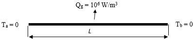
The analysis of non-linear heat flow in a rod with temperature-dependent thermal conductivity is done. There is no loss of heat as shown in Fig. 1 from its surfaces and ends of the rod are maintained at equal temperature $(T_a = T_b = 0^oC)$. Heat is produced at a volumetric rate of $Q_g$.
Relevant parameters used in the analysis are listed in Table 1. The analytical solution of the problem in the steady-state condition is given by (Jiji, 2009):
$ T(x)=\dfrac{-1+\sqrt{1-0.0005\dfrac{Q_g}{k_0}(Lx-x^2)}}{-0.0005} ~~~~~~~~~~~~~~~~~~~~~~~~~~~~~~~~~~~~~~~~ (19)$
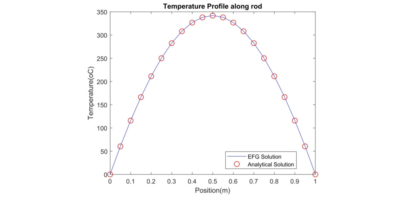
Figure 2shows the temperature profile along the bar computed using EFG along with its analytical result. The result obtained from the EFG method is compared against the results from analytical and FEM solutions at some typical locations in Table 2. This result shows that the EFG method competes well with FEM and has resulted in good agreement with the analytical solution.
This analysis was carried out for the different sizes of the support domain. The size of the support domain (Liu, 2003) is given by the relation:
$ r_s = a_sd_n ~~~~~~~~~~~~~~~~~~~~~~~~~~~~~~~~~~~~~~~~~~~~~~~~~~~~~~~~~~~~~~~~~~~~~~~~~~~~~~~~~~~~~~~~~~~~~~~ (20)$
where,
$ \begin{aligned}
r_s & : \text { The radius of support domain } \\
α_s & : \text { Scaling parameter } \\
d_n & : \text { The characteristic length between nodes }
\end{aligned} $
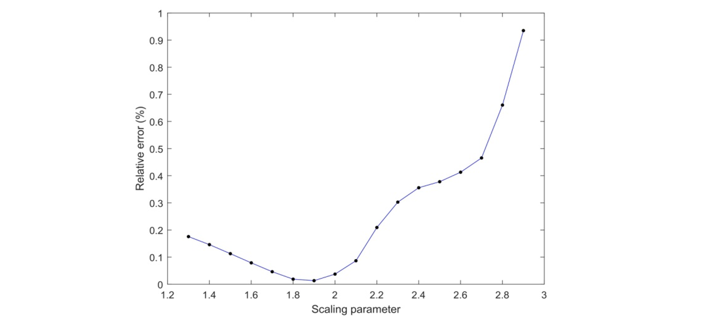
The values of relative error based on $L_2$ norm is plotted in Fig. 3 with respect to the scaling parameter of the corresponding domain. The values of relative error are less for any value of $α_s$ between 1.8 and 2.0 which can be used to obtain more accurate results than the conventional mesh-based method. Larger size of the support domain may not maintainthe local characteristics of the approximation which could deviate the resulting solutions from its true value as seen in the plot, especially for the value of $α_s > 2.0$.
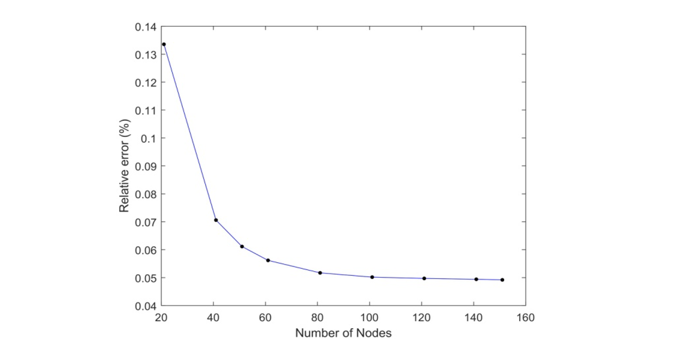
Relative error is also calculated with the increasing number of nodes. It is observed that with the increase in the number of nodes in the domain the value of relative error decreases (Fig. 4). This indicates that EFG has good convergence behavior.
| Parameter | Values |
|---|---|
| Length (L) | 1 m |
| Thermal conductivity (k) | k (T) = k0 (1-0.0005T) k0 = 400 W/m◦C |
| Uniform heat (Qg) | 106 W/m3 |
| Temperature (oC) | |||
|---|---|---|---|
| Position x (m) | Exact | FEM | EFG |
| 0.2 | 211.14 | 211.13 | 211.16 |
| 0.3 | 282.44 | 282.40 | 252.46 |
| 0.4 | 326.67 | 326.60 | 326.70 |
| 0.5 | 341.68 | 341.59 | 341.70 |
Conclusion
The EFG method can be used to solve non-linear steady-state heat conduction problems using the penalty method to enforce essential boundary conditions. The selection of the size of the support domain plays important roles while solving any problem using the meshfree method. It is observed from error analysis that the value of scaling parameter (αs) between 1.8 and 2.0 provides more favorable solutions. With proper selection of support domain, EFG can provide numerical solution of nonlinear heat conduction problem with higher accuracy than other conventional mesh-based methods. This method can be used as an alternative to FEM to solve different nonlinear problems.
Author Details
1Department of Mechanical Engineering, Pulchowk Campus, Institute of Engineering, Tribhuvan University, Nepal
References
Belytschko, T., Y.Y. Lu and L. Gu, 1994. Element-free galerkin methods. Int. J. Numer. Method. Eng., 37(2): 229-256.
Belytschko, T., D. Organ and C. Gerlach, 2000. Element-free galerkin methods for dynamic fracture in concrete. Comput. Method. Appl. M., 187(3-4): 385-399.
Cordes, L.W. and B. Moran, 1996. Treatment of material discontinuity in the element-free galerkin method. Comput. Method. Appl. M., 139: 75-89.
Dai, B., B. Zheng, Q. Liang and L. Wang, 2013. Numerical solution of transient heat conduction problems using improved meshless local Petrov-Galerkin method. Appl. Math. Comput., 219(19): 10044-10052.
Donea, J. and S. Giuliani, 1974. Finite element analysis of steady-state nonlinear heat transfer problems. Nucl. Eng. Des., 30(2): 205-213.
Gingold, R.A. and J.J. Monaghan, 1977. Smoothed particle hydrodynamics: Theory and application to non-spherical stars. Mon. Not. R. Astron. Soc., 181(3): 375-389.
Jiji, L.M., 2009. Heat Conduction. Springer-Verlag, Berlin.
Krysl, P. and T. Belytschko, 1996. Analysis of thin shells by the element-free Galerkin method. Int. J. Solids Struct., 33(20-22): 3057-3080.
Lancaster, P. and K. Salkauskas, 1981. Surfaces generated by moving least squares methods. Math. Comput., 37(155): 141-158.
Liu, G.R., 2003. Meshfree Methods Moving Beyond the Finite Element Method. 2nd Edn., CRC Press.
Liu, W.K., Y. Chen, C.T. Chang and T. Belytschko, 1996. Advances in multiple scale kernel particle methods. Comput. Mech., 18: 73-111.
Nayroles, B., G. Touzot and P. Villon, 1992. Generalizing the finite element method: Diffuse approximation and diffuse elements. Comput. Mech., 10(5): 307-318.
Shepard, D., 1968. A two-dimensional interpolation function for irregularly-spaced data. Proceeding of the 23rd ACM National Conference (ACM ’68), pp: 517-524.
Singh, I.V., 2004. A numerical solution of composite heat transfer problems using meshless method. Int. J. Heat Mass Tran., 47(10-11): 2123-2138.
Thakur, H., 2010. Meshless Local Petrov-Galerkin Method for Phase Change Problems. Indian Institute of Technology, Roorkee.
Wendland, H., 1995. Piecewise polynomial, positive definite and compactly supported radial functions of minimal degree. Adv. Comput. Math., 4(1): 389-396.
Rights and permissions
Open Access: This article is licensed under a Creative Commons Attribution 4.0 International License, which permits use, sharing, adaptation, distribution and reproduction in any medium or format, as long as you give appropriate credit to the original author(s) and the source, provide a link to the Creative Commons license, and indicate if changes were made. The images or other third-party material in this article are included in the article’s Creative Commons license, unless indicated otherwise in a credit line to the material. If material is not included in the article’s Creative Commons license and your intended use is not permitted by statutory regulation or exceeds the permitted use, you will need to obtain permission directly from the copyright holder. To view a copy of this license, visit http://creativecommons.org/licenses/by/4.0/
Cite this Article
Nawraj Bhattarai, Puspa Baral and Ajay Kumar Jha, 2021. Non-Linear Steady State Heat Conduction using Element-Free Galerkin Method. Research Journal of Applied Sciences, Engineering and Technology 18: 20-25 http://doi.org/10.19026/rjaset.18.6061
Received
Accepted
Published
April 15, 2020
May 9, 2020
March 25, 2021
DOI: http://doi.org/10.19026/rjaset.18.6061
Sections
Abstract
Keywords
Introduction
Methodology
Element-free Galerkin method
Meshfree approximation
Moving least square approximation
Weight function
Enforcement of essential boundary conditions
Discrete equation
EFG formulation
Solution of the non-linear system
Results And Discussion
Conclusion
Author Details
References
Rights And Permissions
Cite This Article