Alexander, J.C. and J.H. Maddocks, 1989. On the kinematics of wheeled mobile robots. Int. J. Robot. Res., 8(5): 15-27.
Modeling and Nonlinear Adaptive Control for Omnidirectional Mobile Robot
Research Journal of Applied Sciences, Engineering and Technology 2021 18: 59-69
Cite This ArticleAbstract
This study presents a complete model for RobotinoMD an omnidirectional mobile robot. This model includes the kinematics and dynamics. It is used for the simulation and design of an adaptive nonlinear control system. The hierarchical control system that is proposed has three levels. The level-one which is the inner loop is used to control the DC motors that drive the robot wheels. A control design method combining an adaptive feedback linearization technique and the Backstepping approach is used to find the controller equation. The adaptation module that is included in the control system maintains the performance of the system in the presence of uncertainties on the inertia, weight and other parameters in the robot dynamics. The level-one controller receives its reference signal from the level-two controller which converts the linear and rotational speeds into desired speeds. This level-two controller receives its reference signal from the level-three controller which is the outer loop controller. The level-three controller equation is found so that the robot can follow a desired path described in a Cartesian space. The proposed control system is evaluated in simulation in the MATLAB-SIMULINK environment. It is compared to a PID controller. Simulation results show that the nonlinear adaptive controller has better performances.
Keywords:
Introduction
Mobile robots are increasingly used in industrial and house-hold applications, especially when flexible motions are required on smooth surfaces. Several configurations exist. One distinguishes unicycle, tricycle and omnidirectional mobile robots (Alexander and Maddocks, 1989). An omnidirectional mobile platform is more suitable than a conventional mobile robot with ordinary wheels, for instance for homecare, office and nursing robots. Compared to two or fourth-wheels conventional mobile platforms, it is ease for an omnidirectional mobile robot with three degrees of freedom to move toward the desired direction and the desired orientation (Campion et al., 1996) simultaneously.
The Research Laboratory LARTESY of ENSET-Gabon has recently acquired a Robotino® an omnidirectional mobile robot. The robot is equipped with a manipulator arm which allows it to perform several industrial tasks. The aim of this acquisition is to develop a domestic expertise in advanced robotics. It is within this agenda that the work presented in this study focuses on the modeling and design of an effective control system for Robotino. We will limit ourselves to a validation by simulations. An experimental validation will follow in a near future.
The literature review reveals that several laboratories are working on similar robots. Indeed (Paromtchik and Rembold, 1994) proposes a control system based exclusively on the kinematic model. PID controllers are used to move the robot at a desired speed. In (Kalmár-Nagy et al., 2002), authors take into account both kinematics and dynamics for the design. However, they ignore the coupling between the linear velocity and the rotational speed. A simplified model is therefore used for the robot model. Samani et al., 2004 proposes a control system for an optimal trajectory tracking. However, the angular orientation is not considered in the paper. In (Kalmár-Nagy et al., 2004) authors use two PIDs to control the robot position and orientation simultaneously. A simplified model is also used for the robot model. Watanabe et al., 1998 uses PI and PD to control the speed and orientation of the robot. The control system is tested in practice. Dixon et al., 2000 proposes a variable- structure control system for the omnidirectional mobile robot.
This study presents a complete modeling of an omnidirectional mobile robot. The model includes the robot kinematics and dynamics. It will be used to develop the simulation file and to design the control system for the robot. A hierarchical control system is proposed. It has three levels. The level one directly controls DC motors that rotate robot wheels. The level two is used to convert the desired robot linear and rotational speeds into desired wheel speeds. The level three is used to generate the desired robot linear and rotational speeds so that the robot can follow a desired path specified in a Cartesian space. It will be assumed that parameters that appear in the robot model are not known. This assumption is realistic since the model depends on inertia and mass. These parameter values are generally not provided by the manufacture. A module that will automatically adjust controller parameters will be integrated to the control system so that good performances can be achieved even though robot parameters are unknown. The contribution of paper is the design of a multivariable adaptive nonlinear control law for the controller at the level 1 of the proposed hierarchical control system.
Materials And Methods
This study was conducted at the Research Laboratory LARTESY of ENSET-Gabon. The paper proposes a novel control system for the wheels of an omnidirectional mobile robot. The controller is at the level one of a three-level hierarchical control system. As a consequence, the design of the hierarchical control system is also given. A model-based design approach is used. Therefore, controller equations are obtained using the mathematical model for the mobile robot.
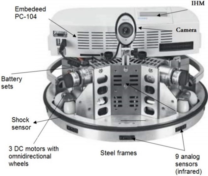
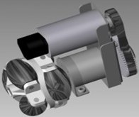
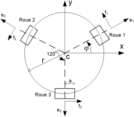
Figure 1 shows RobotinoMD an omnidirectional robot. Figure 2 presents one of the robot wheels. The robot is equipped with a microcomputer that is mainly used to control the wheels. It has three wheels located at 120º apart as illustrated at Fig. 3. Each wheel is driven by a DC motor. Equations that describe the robot position and motion in the Cartesian space will be presented. These equations will be used to find controller equation and to simulate the system in closed loop. It is shown in Angeles, 2003 that linear and rotational speeds for the robot can be written in terms of wheel speeds as follows:
$ \bar V_R = - \dfrac{2a}{3} \sum\limits_{i=1}^3 \omega_i \bar f_i ~~~~~~~~~~~~~~~~~~~~~~~~~~~~~~~~~~~~~~~~~~~~~~~~~~~~~~~~~~~~~~~~~~ (1)$
$ \omega_R = - \dfrac{a}{3r} \sum\limits_{i=1}^3 \omega_i ~~~~~~~~~~~~~~~~~~~~~~~~~~~~~~~~~~~~~~~~~~~~~~~~~~~~~~~~~~~~~~~~~~~~~ (2)$
$ \begin{aligned} \bar f_1 & = \Big(-sin\varphi \;\;\; cos\varphi \Big)^T \\ \bar f_2 & = \Big(-sin \big( \varphi + 120° \big) \;\;\; cos \big( \varphi + 120° \big) \Big)^T \\ \bar f_3 & = \Big(-sin \big( \varphi - 120° \big) \;\;\; cos \big( \varphi - 120° \big) \Big)^T \\ \bar e_1 & = \Big( cos \varphi \;\;\; sin \varphi \Big)^T \\ \bar e_2 & = \Big( cos \big( \varphi + 120° \big) \;\;\; sin \big( \varphi + 120° \big) \Big)^T \\ \bar e_3 & = \Big( cos \big( \varphi - 120° \big) \;\;\; sin \big( \varphi - 120° \big) \Big)^T \end{aligned} ~~~~~~~~~~~~~~~~~~~~~~~~ (3)$
where the variables $ \bar V_R $ and $ ω_R $ designate the linear and rotational speed for the robot, respectively. $ ω_i $ is the rotational speed for the wheel number i. $ φ $ is the angle of orientation for the robot, as indicated in Fig. 3. Parameters $ r $ and a represent the radius for the mobile platform and the wheel, respectively. It should be noted that the rotational speed vector for each wheel $ i $ (i.e., $ \bar ω_i $) is oriented in the direction of the unit vector $ \bar e_i $ as illustrated at Fig. 3.
The linear and rotational speeds can be written in terms of the robot position and orientation in the plane, as follows:
$ \bar V_R = \Big(\dot x_R \;\;\; \dot y_R \Big)^T \;\;\; \omega_R = \dot \phi ~~~~~~~~~~~~~~~~~~~~~~~~~~~~~~~~~~~~~~~~~~~~~~~~~~~ (4)$
where,
$ \begin{aligned}
x_R \; \text {and} \; y_R & : \text {The coordinates of the center of the robot in the Cartesian plane}
\end{aligned} $
Equation (1) and (2) can therefore be rewritten in a matrix form as follows:
$ \begin {pmatrix} \dot x_R \\\ \dot y_R \\\ \dot \varphi \end {pmatrix} = - \dfrac{2a}{3} \begin {bmatrix} -sin\varphi & \frac{1}{2} sin\varphi - \frac {\sqrt3}{2} cos\varphi & \frac{1}{2} sin\varphi + \frac {\sqrt3}{2} cos\varphi \\\ cos\varphi & -\frac{1}{2} cos\varphi - \frac {\sqrt3}{2} sin\varphi & -\frac{1}{2} cos\varphi + \frac {\sqrt3}{2} sin\varphi \\\ 1/(2r) & 1/(2r) & 1/(2r) \end {bmatrix} \begin {pmatrix} \omega_1 \\\ \omega_2 \\\ \omega_3 \end {pmatrix} ~~~~~~~~~~~~~~~~~~~~~~~~ (5)$
Equation (5) is the robot kinematics. Since the robot displacement is significantly impacted by its mass and inertia, its dynamic model is considered for the design of the controller. The following are the robot dynamic equations. They show the relationships between wheel accelerations and applied torques:
$ J_R \begin {pmatrix} \dot \omega_1 \\\ \dot \omega_2 \\\ \dot \omega_3 \end {pmatrix} + C(\omega_R) \begin {pmatrix} \omega_1 \\\ \omega_2 \\\ \omega_3 \end {pmatrix} = \begin {pmatrix} \tau_1 \\\ \tau_2 \\\ \tau_3 \end {pmatrix} - D_R \begin {pmatrix} \omega_1 \\\ \omega_2 \\\ \omega_3 \end {pmatrix} ~~~~~~~~~~~(6)$
where,$ \begin{aligned} J_R \; \text {and} \; D_R & : \text {The inertia and the friction coefficient for the wheels, respectively} \\ C(\omega_R) & : \text {Includes Coriolis terms and it is given below} \\ \tau_i \; i = 1, 2, 3 & : \text {Electric torques applied to the wheels by the DC motors} \end{aligned} $
Torque equations will be obtained later in this section:
$ \begin{aligned} C(\omega_R) & = 2 \sqrt3 \left( \frac{a}{3r} \right)^2 \left(3m_w + m_p \right) r\omega_R \begin {bmatrix} 0 & -1 & 1 \\\ 1 & 0 & -1 \\\ -1 & 1 & 0 \end {bmatrix} \\ J_R & = \begin {bmatrix} \alpha & \beta & \beta \\\ \beta & \alpha & \beta \\\ \beta & \beta & \alpha \end {bmatrix} \end{aligned} ~~~~~~~~~~~~~~~~~~~~~~~~~~~~~~~~~ (7)$
where,
$ \begin{aligned} \alpha & = I + \left( \frac {a}{3r} \right)^2 \left\{ H + 3J + 15m_wr^2 + 3m_pr^2 \right\} \\ \beta & = \left( \frac {a}{3r} \right)^2 \left\{ H + 3J + 3m_wr^2 + 3m_pr^2 \right\} \;\; I_w = \begin {bmatrix} I & 0 & 0 \\\ 0 & J & 0 \\\ 0 & 0 & J \end {bmatrix} \end{aligned} ~~~~~~~~~~~~~~~~~~~~~~~~~~ (8)$
Numerical values for parameters that appear in (8) are provided in Table 1. Equation (6) is detailed as follows:
$ \begin{aligned} \dot \omega_1 & = C \Big(\omega_1 + \omega_2 + \omega_3 \Big) \Delta_1 - D \Big(A\omega_1 + B\omega_2 + B\omega_3 \Big) + K_t \Delta_0 \\ \dot \omega_2 & = C \Big(\omega_1 + \omega_2 + \omega_3 \Big) \Delta_2 - D \Big(A\omega_1 + B\omega_2 + B\omega_3 \Big) + K_t \Delta_0 \\ \dot \omega_3 & = C \Big(\omega_1 + \omega_2 + \omega_3 \Big) \Delta_3 - D \Big(A\omega_1 + B\omega_2 + B\omega_3 \Big) + K_t \Delta_0 \end{aligned} ~~~~~~~~~~~~~~~~~~~~~~~~~~ (9)$
where,
$ \begin{aligned} \Delta_0 & = \Big(AI_1 + BI_2 + BI_3 \Big) \\ \Delta_1 & = A \Big(\omega_3 - \omega_2 \Big) + B \Big(\omega_1 - \omega_3 \Big) + B \Big(\omega_2 - \omega_1 \Big) \\ \Delta_2 & = B \Big(\omega_3 - \omega_2 \Big) + A \Big(\omega_1 - \omega_3 \Big) + B \Big(\omega_2 - \omega_1 \Big) \\ \Delta_3 & = B \Big(\omega_3 - \omega_2 \Big) + B \Big(\omega_1 - \omega_3 \Big) + A \Big(\omega_2 - \omega_1 \Big) \\ A & = \Big(\alpha^2 - \beta^2 \Big) / \Big(\alpha^3 - 2\beta^3 - 3\alpha \beta^2 \Big) \;\;\; B = \Big(\beta^2 - \alpha\beta \Big) / \Big(\alpha^3 - 2\beta^3 - 3\alpha \beta^2 \Big) \end{aligned} $
The variable Ii is the current for the DC motor i. The DC motor can be described by the following model:
$ L \dfrac {d}{dt} I_i + RI_i = V_{ti} - K_s \omega_i \;\;\; \left( i = 1, 2, 3 \right) ~~~~~~~~~~~~~~~~~~~~~~~~~~~~~~~~~~~~~~~~~~~~~~~~~~~~~~~~~~~~ (10)$
The relationship between the DC motor current and torque is clarified below. L, R and Ks are the inductance for the motor coil, the resistance, and the magneto motive force coefficient respectively. Vti(t) is the armature voltage. The electric torque is denoted τi. It is proportional to the current according to the following relationship:
$ \tau_i = K_t I_i \;\;\; \left( i = 1, 2, 3 \right) ~~~~~~~~~~~~~~~~~~~~~~~~~~~~~~~~~~~~~~~~~~~~~~~~~~~~~~~~~~~~~~~~~~~~~~~~~~~~~~~~~~~~~~~~~~ (11)$
Kt is the torque coefficient. It is equal to Ks. The omnidirectional robot model consists of Eq. (6), (9) and (10).
The inductance L is usually very small. Therefore, it can be neglected. Equation (10) reduces to the following algebraic equation:
$ I_i = \dfrac{1}{R} V_{ti} - \dfrac{K_\omega}{R} \omega_i \;\;\; \left( i = 1, 2, 3 \right) ~~~~~~~~~~~~~~~~~~~~~~~~~~~~~~~~~~~~~~~~~~~~~~~~~~~~~~~~~~~~~~~~~~~~~~~~ (12)$
Mobile robot control system: This section discusses the structure of the control system for RobotinoMD an omnidirectional mobile. This control system can be divided into three levels. It is therefore a hierarchical system in which the output of an upper level is the input of the following lower level.
The level three consists of a module that will allow the robot to follow a desired path. This path is described in the Cartesian plane. The output of the level three are the linear and rotational speeds that the robot should have to follow the desired path. These desired speeds are then converted into desired rotational wheel speeds. This conversion takes place at level two of the hierarchical structure. Desired wheel speeds are references for the level one controller which directly controls three DC motors. The main contribution of this paper is the design of the level one controller. It is assumed that parameters that appear in Eq. (6) and (10) are unknown or may change when the robot operates. This makes the problem very challenging. The so-called state feedback linearization methodology coupled with the adaptive Backstepping control design method is used to obtain the control and adaptation laws for the level one controller parameters. The following sections present the design of the proposed hierarchical control system.
Equations for the trajectory tracking controller: The level three of the hierarchical control system allows the mobile robot to follow a desired path. This path is given in the Cartesian coordinates in terms of the desired position and orientation of the robot at a given time instance. The output signals of this level three controller are the linear and rotational speeds that the robot should have to accurately follow the desired path.
If $x_R^d\;(t)$ and $y_R^d \; (t)$ denote the x-coordinate and y-coordinate for the robot position in the Cartesian plane and $ \varphi^d (t)$ is the robot orientation; the linear and rotational speeds that the robot should have to follow the path are:
$ \begin{aligned} V^d_x & = -K_x \Big( x_R \big( t \big) - x^d_R \big( t \big) \Big) + x^d_R \big( t \big) \\ V^d_y & = -K_y \Big( y_R \big( t \big) - y^d_R \big( t \big) \Big) + y^d_R \big( t \big) \\ \omega^d & = -K_\omega \Big( \varphi \big( t \big) - \varphi^d \big( t \big) \Big) + \varphi^d \big( t \big) \\ \varphi^d \big( t \big) & = atan2 \Big(y^d_R \;, x^d_R \Big) \;\;\; \varphi^d \big( t \big) = \dfrac {\dot y^d_R \; \dot x^d_R - \ddot y^d_R \;, \ddot x^d_R}{\left( \dot x^d_R \right)^2 + \left( \dot y^d_R \right)^2} \end{aligned} ~~~~~~~~~~~~~~~~~~~~~~~~~~~~~~~~~~~~~~~~~ (13)$
where,
$ \begin{aligned}
V_x^d \; (t), \; V_y^d \; (t) & : \text {Desired linear speed coordinates} \\
\omega^d & : \text {The desired rotational speed for the robot}
\end{aligned} $
The gains $ K_x$, $K_y$ and $K_φ$ are positive real numbers. Equations (13) are control equations for the level three controller. Next section discusses the equation used to convert the desired robot linear speeds into desired rotational wheel speeds.
Equations for the module to converter linear speeds into rotational speeds: The desired linear and rotational robot speeds are converted into wheel speeds that each motor should have for the robot to be able to follow the desired path. This conversion takes place at the level two of the hierarchical control system. The robot kinematics described at Eq. (5) is used to perform this conversion. For a given robot speed vector, the wheel speed vector is obtained by inverting the robot kinematics. This yields to the following desired wheel speed expressions:
$ \begin {pmatrix} \omega_{1d} \\\ \omega_{2d} \\\ \omega_{3d} \end {pmatrix} = M^{-1} \begin {pmatrix} V^d_x \\\ V^d_y \\\ \omega^d \end {pmatrix} ~~~~~~~~~~~~~~~~~~~~~~~~~~~~~~~~~~~~~~~~~~~~~~~~~~~~~~~~~~~~~~~~~~~~~~~~~~~~~~~~~~~~~~~~~ (14)$
$ M = - \dfrac{2a}{3} \begin {bmatrix} -sin\varphi & \frac{1}{2} sin\varphi - \frac {\sqrt3}{2} cos\varphi & \frac{1}{2} sin\varphi + \frac {\sqrt3}{2} cos\varphi \\\ cos\varphi & -\frac{1}{2} cos\varphi - \frac {\sqrt3}{2} sin\varphi & -\frac{1}{2} cos\varphi + \frac {\sqrt3}{2} sin\varphi \\\ 1/(2r) & 1/(2r) & 1/(2r) \end {bmatrix} ~~~~~~~~~~~~~~~~~~~~ (15)$
Equation (14) is the control equation for the level two controller. The next section discusses how the control system at the level one uses the desired wheel speed information to effectively control the three DC motors.
Equations for DC motor controllers: The last level of the hierarchical control system consists of controllers for each of the three robot wheels. The objective of these controllers is to ensure that each wheel rotates at its desired speed which is provided by the level two of the hierarchical structure. It is worth mentioning that the desired speed is a time varying signal. A model-based control design method that uses the robot dynamic equations is proposed to find the controller equation. The advantage of this design approach is that it takes into consideration interactions between different components of the mobile robot. As a consequence, the performance of the control system is excellent.
Dynamic equations for the wheels and motors are described by Eq. (9) and (10) respectively. A Backstepping control design method is used to find the equation for $V_{ti}(t)$ that will ensure that the speed $ω_i(t)$ follows its desired value. This design scheme has two steps. First, the expression for $I_i^*(t)$ is obtained. It’s the value the DC motor current $I_i(t)$ should have to guarantee that the DC motor speed $ω_i(t)$ converges asymptotically to its desired value $ω_{id}(t)$. Next, the motor input voltage equation $V_{ti}(t)$ is obtained. The voltage is such that the motor current $I_i(t)$ converges asymptotically to its reference $I_i^*(t)$. The system dynamics can be written into a closed form as follows:
$ \dot {\bar \omega} = f_\omega \left( \bar \omega , \bar \theta_1 \right) + g_\omega \left( \bar \omega , \bar \theta_1 \right) \bar I ~~~~~~~~~~~~~~~~~~~~~~~~~~ (16)$
$ \dot {\bar I} = f_I \left( \bar \omega , \bar I , \bar \theta_2 \right) + g_I \left(\bar \theta_2 \right) \bar V_t ~~~~~~~~~~~~~~~~~~~~~~~~~~ (17)$
Where functions and variables that appear in above equations are defined as follows:
$ \bar \omega = \left( \omega_1, \omega_2 , \omega_3 \right)^T \;\;\; \bar I = \left( I_1, I_2 , I_3 \right)^T \;\;\; \bar V_t = \left( V_{t1}, V_{t2} , V_{t3} \right)^T $
$ \bar \theta_1 = \left( AC_c, BC_c, AD, BD, AK_t, BK_t \right)^T \;\;\; \bar \theta_2 = \left( R/L, K_s/L, I/L \right)^T $
$ f_\omega = \begin {bmatrix} C_c \Big(\omega_1 + \omega_2 + \omega_3 \Big) \Delta_1 - D \Big(A\omega_1 + B\omega_2 + B\omega_3 \Big) \\\ C_c \Big(\omega_1 + \omega_2 + \omega_3 \Big) \Delta_2 - D \Big(B\omega_1 + A\omega_2 + B\omega_3 \Big) \\\ C_c \Big(\omega_1 + \omega_2 + \omega_3 \Big) \Delta_3 - D \Big(B\omega_1 + B\omega_2 + A\omega_3 \Big) \end {bmatrix} \;\;\; g_\omega = K_k \begin {bmatrix} A & B & B \\\ B & A & B \\\ B & B & A \end {bmatrix} $
$ f_I = \begin {bmatrix} -R/LI_1 - K_s/L\omega_1 \\\ -R/LI_2 - K_s/L\omega_2 \\\ -R/LI_3 - K_s/L\omega_3 \end {bmatrix} \;\;\; g_I = K_k \begin {bmatrix} 1/L & 0 & 0 \\\ 0 & 1/L & 0 \\\ 0 & 0 & 1/L \end {bmatrix} $
It will be assumed that parameter vectors $ \bar \theta_1$ and $\bar \theta_2$ are constant but their values are unknown to the control designer. For design purposes, let us consider $\widetilde{\bar \omega} = \bar \omega - \bar \omega_d$ the error between wheel speeds vector and its reference $ \bar \omega_d = \left(\omega_{d1}, \omega_{d2}, \omega_{d3} \right)^T$ The dynamic equation for the error has therefore the following form:
$ \dot {\widetilde \omega} = f_\omega \left( \bar \omega , \hat {\bar \theta_1} \right) + g_\omega \left( \bar \omega , \hat {\bar \theta_1} \right) \bar I - \dot {\bar \omega_d} \left( t \right) + h_\omega \left( \bar \omega , \bar I \right) \tilde {\bar \theta_1} ~~~~~~~~~~~~~~~~~~~~~~~~~~~~~~~~~~~~~~ (18)$
Where $\tilde{\bar \theta_1} = \bar \theta_1 - \hat {\bar \theta_1}$ is the error between the vector of unknown parameters $ \bar \theta_1$ and its estimate $\hat{\bar \theta_1}$. It’s worth mentioning that $\hat{\bar \theta_1}$ a vector of controller parameters. If the motor currents vector $\bar I(t)$ were the control signal, it would suffice to choose its expression, as follows, for the velocity error vector $\widetilde{\bar \omega}$ to converge to zero asymptotically:
$ \bar I^* = g_\omega^{-1} \left( \bar \omega , \hat {\bar \theta_1} \right) \Big \{ -f_\omega \left( \bar \omega , \hat {\bar \theta_1} \right) + \dot {\bar \omega_d} \left( t \right) + A_\omega \widetilde {\bar \omega} \Big \}~~~~~~~~~~~~~~~~~~~~~~~~~~~~~~~~~~~~~~~~~~~~ (19)$
$A\omega$ is a Hurwitz diagonal matrix. Equation (19) is such that it compensates the nonlinear terms in Eq. (18) and it stabilizes the speed error dynamic equation. Note that Eq. (19) includes $\hat {\bar \theta_1}$ which is provided by the adaptation module yet to be designed. The equation that describes how $\hat {\bar \theta_1}$ is computed will be discussed later.
However, $\bar I(t)$ is not the true control signal. As a consequence, Eq. (19) will be used to define a new variable $\hat{\bar I}(t)$ which is the difference between $\bar I(t)$ and its reference $I^*_i(t)$. Substituting Eq. (19) in (18) and defining the new current error variable $\tilde{\bar I}(t)$ yields, Eq. (20). This equation is important to show the stability of the closed loop system and to find the equation for the adaptation module:
$ \dot {\widetilde {\bar \omega}} = A_\omega \widetilde {\bar \omega} + g_\omega \left( \bar \omega , \hat {\bar \theta_1} \right) \tilde {\bar I} + h_\omega \left( \bar \omega , \bar I \right) \tilde {\bar \theta_1} ~~~~~~~~~~~~~~~~~~~~~~~~~~~~~~~~~~~~~~~~~~~~~~~~~~~~~~~~~~~~~~~~ (20)$
The dynamic equation for the new variable has the following form:
$ \begin{aligned} \dot {\tilde {\bar I}} & = f_1 \left( \bar \omega, \bar I, \hat {\bar \theta_2} \right) + g_1 \left( \hat {\bar \theta_2} \right) \bar V_t + h_1 \left( \bar \omega , \bar I \right) \tilde {\bar \theta_2} \\ & - \dfrac {\partial \bar I^*} {\partial \hat {\bar \theta_1}} \dot {\hat {\bar \theta_1}} - \dfrac {\partial \bar I^*} {\partial \bar \omega} \Big \{ f_\omega \left( \bar \omega , \hat {\bar \theta_1} \right) + g_\omega \left( \bar \omega, \hat {\bar \theta_1} \right)\bar I + h_\omega \left( \bar \omega, \bar I \right) \tilde {\bar \theta_1} \Big \} \end{aligned} ~~~~~~~~~~~~~~~~~~~~~~~~ (21)$
Equation (21) is used to find the expression for the true control signal so that the error variable converges to zero asymptotically. The equation for the level one is therefore:
$ \begin{aligned} \bar V_t & = g^{-1}_I \left( \hat {\bar \theta_2} \right) \Bigg \{ \dfrac {\partial \bar I^*} {\partial \hat {\bar \theta_1}} \dot {\hat {\bar \theta_1}} + \dfrac {\partial \bar I^*} {\partial \bar \omega} \bigg[ f_\omega \left( \bar \omega , \hat {\bar \theta_1} \right) + g_\omega \left( \bar \omega, \hat {\bar \theta_1} \right)\bar I \bigg ] \Bigg \} \\ & + g^{-1}_I \left( \hat {\bar \theta_2} \right) \Big \{ A_1 \tilde I - P^{-1}_2 P_1 g_\omega \left( \bar \omega, \hat {\bar \theta_1} \right) - \tilde {\bar \omega} f_I \left( \bar \omega, \bar I, \hat {\bar \theta_2} \right) \Big \} \end{aligned} ~~~~~~~~~~~~~~~~~~~~~~~~~ (22)$
The matrix AI is a Hurwitz diagonal matrix. Substituting Eq. (22) in (21), we obtain the following equation which is useful to show the stability of the system in closed loop:
$ \begin{aligned} \dot {\tilde {\bar I}} & = A_1 \tilde {\bar I} - P^{-1}_2 P_1 g_\omega \left( \bar \omega, \hat {\bar \theta_1} \right) \tilde {\bar \omega} + h_\omega \left( \bar \omega, \bar I \right) \tilde {\bar \theta_2} \\ & - \dfrac {\partial \bar I^*} {\partial \bar \omega} h_\omega \left( \bar \omega, \bar I \right) \tilde {\bar \theta_1} \end{aligned} ~~~~~~~~~~~~~~~~~~~~~~~~~~~~~~~~~~~~~~~~~~~~~~~~~~~~~ (23)$
Equation (23) includes the estimated parameter $\hat {\bar \theta_2} $. This parameter is provided by the adaptation module. It is proposed to compute $\hat {\bar \theta_1} $ and $\hat {\bar \theta_2} $ from the Eq. (24) which is the adaptation law:
$ \begin{aligned} \dot {\hat {\bar \theta_1}} & = \Gamma_1 \Bigg \{ h_\omega \left( \bar \omega, \bar I \right)^T P_1 \tilde {\bar \omega} - \left( \dfrac {\partial \bar I^*} {\partial \bar \omega} h_\omega \left( \bar \omega, \bar I \right) \right)^T P_2 \tilde {\bar I} \Bigg \} \\ \dot {\hat {\bar \theta_1}} & = \Gamma_2 \Bigg \{ h_1 \left( \bar \omega, \bar I \right)^T P_2 \tilde {\bar I} \Bigg \} \end{aligned} ~~~~~~~~~~~~~~~~~~~~~~~~~~~~~~~~~~~~~~~~~ (24)$
The adaptation law is the equation for the adaptation module. It is possible to show that Eq. (24) along with Eq. (22) ensure that robot wheel speeds converge to their desired values. For this purpose, we define the following Lyapunov candidate function:
$ V = {\widetilde {\bar \omega}}^T P_1 \widetilde {\bar \omega} + {\tilde {\bar I}}^T P_2 \tilde {\bar I} + {\tilde {\bar \theta_1}}^T \Gamma_1^{-1} \tilde {\bar \theta_1} + {\tilde {\bar \theta_2}}^T \Gamma_2^{-1} \tilde {\bar \theta_2} ~~~~~~~~~~~~~~~~~~~~~~~~~~~~~~~~~~~~~~~~~~~~~~~~~~~~ (25)$
where,
$ \begin{aligned}
\Gamma_1 \; \text {and} \; \Gamma_2 & \; : \; \text {Positive definite matrices} \\
P_1 \; \text {and} \; P_2 & \; : \; \text {Positive definite matrices that satisfy the following relationships} \\
& \; \; \; \; A_{\omega}^T P_1 + P_1 A_{\omega}= - Q_1, \; A_1^T P_2 + P_2 A_1= - Q_2 \; \text{and} \; Q_1, Q_2 \gt 0
\end{aligned} $
The Lyapunov function is positive definite and its derivative has the following form:
$ \begin{aligned} \dot V & = - {\widetilde {\bar \omega}}^T Q_1 \widetilde {\bar \omega} + {\tilde {\bar I}}^T Q_2 \tilde {\bar I} + 2 \tilde {\bar \theta_2}^T \Bigg \{ \Gamma_2^{-1} \dot {\tilde {\bar \theta_2}} + h_I \left( \bar \omega, \bar I \right)^T P_2 \tilde {\bar I} \Bigg \} \\ & = + 2 \tilde {\bar \theta_1}^T \Bigg \{ \Gamma_1^{-1} \dot {\tilde {\bar \theta_1}} + h_\omega \left( \bar \omega, \bar I \right)^T P_1 \tilde {\bar \omega} - \left( \dfrac {\partial \bar I^*} {\partial \bar \omega} h_\omega \left( \bar \omega, \bar I \right) \right)^T P_2 \tilde {\bar I} \Bigg \} \end{aligned} ~~~~~~~~~~~~~~~~~~~~ (26)$
Substituting Eq. (24) in (26) yields:
$ \dot V = - {\widetilde {\bar \omega}}^T Q_1 \widetilde {\bar \omega} - {\tilde {\bar I}}^T Q_2 \tilde {\bar I} \leq 0 ~~~~~~~~~~~~~~~~~~~~~~~~~~~~~~~~~~~~~~~~~~~~~~~~~~~~~~~~~~~~~~~~~~~~~~~~~~~~~~~~~~ (27)$
The derivative of the Lyapunov candidate function is therefore semi-negative definite. One can conclude that the system represented by Eq. (20), (21) and (24) is stable (Marino and Tomei, 1996). The quadratic function represented by Eq. (25) is a Lyapunov function for the system. As a consequent, system variables are bounded. The Barbalat Lemma can be used to show that the system state variables converge to zero asymptotically (Marino and Tomei, 1996). The proposed control system allows the robot to follow (after a short transient period) a desired path. The proposed controller is evaluated in simulation in the next section. It should be noted that the adaptive control law proposed for the level one control system has never been proposed before for an omnidirectional robot. This adaptive controller is the main contribution of the paper.
| Physical variables | Values |
|---|---|
| Robot radius | r = 0.175 m |
| Wheel radius | a = 0.04 m |
| Robot mass | Mp = 11 kg |
| Motor mass | Mm = 0.39 kh |
| Wheel mass | Mr = 1.11 kg |
| Wheel inertia | I = 0.0018 |
| Motor inertia | J = 0.0853 |
| Robot inertia | H = 0.3369 |
| Damping coefficient | D = 0 |
| Torque coefficient | Kt = 0.8 |
| Resistance | R = 26.67 Ω |
| Inductance | L = 0.0011 H |
Results And Discussion
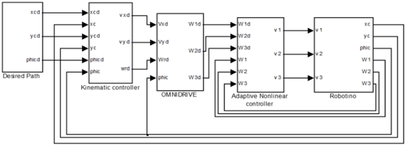
Parameters for Robotino from the LARTESY laboratory of ENSET-Gabon are used to develop the mathematical model for an omnidirectional mobile robot. The model is used to design an adaptive nonlinear controller that will be simulated in this section. The objective is to validate that the control system effectively allows the robot to follow a given trajectory. The performance of the proposed controller will be compared to that of a three-level hierarchical control system consisting of PIDs at levels one and three. The control module at level 2 in both control systems are the same. This module is used to convert robot speeds into wheelspeeds. First, we assume that robot parameters are known. Therefore, the adaptation module is turned off and the level one controller is a non-adaptive nonlinear controller. The simulation file is developed in MATLAB-SIMULINK. Figure 4 below shows the components of this simulation file. The module representing the mobile robot can easily be identified. It is the 'Robotino' module. This module contains Eq. (5), (9) and (10). The path to be followed is generatedbythe 'Desired Path' module. The hierarchical control system is represented by the 'Kinematic Controller' module for level three controller, the 'OMNIDRIVE' module for level two controller and the 'Adaptive Nonlinear Controller' module for level on control system.
Robot parameters and controller gains are given in Table 1 to 3. The desired path that the robot needs to follow is a circle with a radius Rt = 1 m. The robot is initially located at (x = 0.5 m and y = 0.5 m). The desired trajectory begins at t = 0 at (x = 0, y = 0). The performance criterion is the capability of the robot to reach the desired trajectory quickly. The circular trajectory equation is:
$ \begin{aligned} x_d (t) & = R_t \Big \{ 1 - cos \left ( 2 \pi t/T \right ) \Big \} \\ y_d (t) & = R_t sin \left ( 2 \pi t/T \right ) \\ \varphi (t) & = 0 \end{aligned} ~~~~~~~~~~~~~~~~~~~~~~~~~~~~~~~~~~~~~~~~~~~~~~~~~~~~~~~~~~~~~~~~~~~~~~~~~~~~~~~ (28)$
where,
$ \begin{aligned}
R_t & : \text {The path radius} \\
T & : \text {The time required to travel the path}
\end{aligned} $
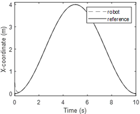
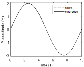
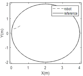
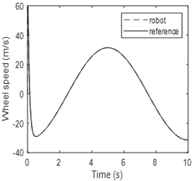
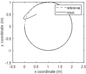
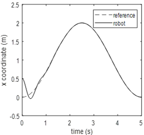
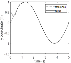
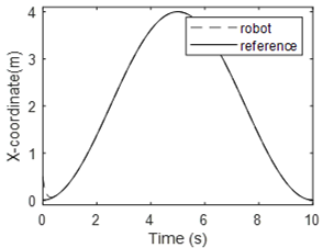
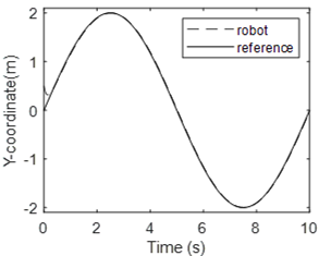
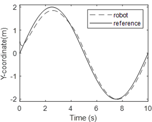
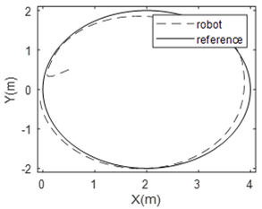
Simulation results are given in Fig. 5 to 8 for the non-linear control system and in Fig. 9 to 11 for the PID controller. Figure 5 illustrates the x-coordinate positions for the robot and the desired trajectory. It is easy to see that therobot reaches the desired trajectory in 0.5 sec without overshoot. The steady-state error is negligible. The trajectory tracking performance for the proposed controller is therefore perfect after 0.5 sec. Figure 6 illustrates the y-coordinate positions for the robot and desired trajectory. The same conclusion regarding the tracking performance can be made for the nonlinear control system. Figure 7 represents the robot position in the x-y plane. This figure is a picture of the robot when it is moving in a two-dimensional space. It shows clearly that the circle drawn by the robot and the desired circle are identical. Fig. 8 shows the wheel speed waveform. It should be noted that this speed remains within the limits allowed by the robot.
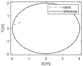
Figure 9 to 11 illustrate the waveforms when level one and three controllersare PIDs. Figure 9 represents the robot position and the desired circular path in thex-y plane. One can see that the robot can barely follow the desired trajectory. This underperformance can be seen in Fig. 10 and 11 which show the x-coordinate and y-coordinate for the robot and the desired path.
One can conclude that the proposed nonlinear control system for the omnidirectional robot is much better than the conventional PID controller. The main reason for this performance is that the robot has a highly coupled nonlinear model and the best control system for these dynamics is a nonlinear controller which takes into consideration the coupling between robot components. The proposed control system decouples these dynamics to be able to control the robot efficiently.
Next, capabilities of the proposed control system to maintain the same good performance despite changes on robot parameters are tested. For this test, the robot moves from a smooth surface to a rough surface. As a consequence, the parameter D in the Eq. (9) changes significantly. This causes an uncertainty on the value for third and fourth elements in the parameter vector $ \bar \theta_1 $. The other parameters remain constant and known. A comparative study will be carried out between the adaptive control system and its non-adaptive version. The robot will travel the desired trajectory when it is controlled by the nonlinear control system with the adaptation module activated, and when the adaptive module is not activated. The desired trajectory is a circle which begins at the (x = 0, y = 0). The robot is initially positioned at (x = 0.5 m, y = 0.5 m).
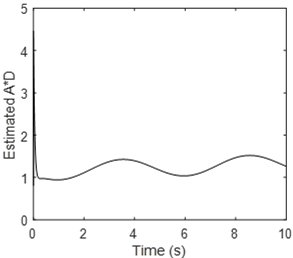
Simulation results when the adaptive module is activated are shown in Fig. 12 to 15. Figure 12 illustrates the robot position and the desired trajectory in the x-y plan. It is easy to see that the robot follows the desired trajectory after a short transient period. The performance is almost identical to the previous case. It can therefore be concluded that the adaptive module allows the control system to maintain its performance despite uncertainties in robot model parameters. Figure 13 and 14 show the x-coordinate and y-coordinate waveforms for the robot and the desired path. It can be noted that the tracking error is almost zero. Figure 15 shows one of the waveformsfor an estimated parameter. It’s the waveform for the third element in the parameter vector $ \bar \theta_1 $. This figure demonstrates that the estimated parameter remains bounded. Simulation results show that the mainobjective of this study is met. Indeed, the proposed controller is nonlinearand it is able to control the robot although robot parameters are completely unknown.
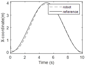
Figure 16 to 18 illustrate the simulation result when the adaptive module is deactivated. In this context, controller parameters are initialized with values that are not necessarily the true values. Figure 16 shows the x-coordinate waveform and Fig. 17 illustrates the y-coordinate waveform. It can easily be noted that the robot has some difficulties in following the desired coordinates. Tracking errors are much bigger. Figure 18 shows the two-dimensional movement of the robot. It provides an overview of the control system performance when model parameters are not perfectly known. This figure demonstrates that an adaptive module is necessary for the control system to have a good performance when model parameters are uncertain.
| Gains | Values |
|---|---|
| Level 3 controller gain | $K_x = K_y = K_φ = 10$ |
| Level 1 controller gain matrix | $ A_w = \begin{bmatrix} -100 & 0 & 0\cr 0 & -100 & 0\cr 0 & 0 & -100 \end{bmatrix} $ |
| Level 1 controller gain matrix | $ A_I = \begin{bmatrix} -1000 & 0 & 0\cr 0 & -1000 & 0\cr 0 & 0 & -1000 \end{bmatrix} $ |
| Gains | Values |
|---|---|
| Proportinal gain $ K_p $ | 10 |
| Integral gain $ K_i $ | 100 |
| Derivative gain $ K_d $ | 1 |
Conclusion
A three-level hierarchical adaptive nonlinear control system is proposed for an omnidirectional mobile robot. The advantage of the proposed approach is that it allows taking into account robot highly coupled nonlinear dynamic equations to design suitable and therefore efficient control laws. A module that updates controller parameters is used to significantly reduced the sensitive of the proposed control system to parameter uncertainties. The performance of the proposed control system is evaluated in simulation. It is also compared to a conventional PID controller. Simulation results show that that the adaptive nonlinear control system allows the mobile robot to follow almost perfectly a desired path. The controller keeps the same performance despite significant uncertainties on robot parameters. A practical implementation of this control system is foreseen at the LARTESY laboratory at ENSET-Gabon. The laboratory has recently acquired a RobotinoMD an Omnidirectional mobile robot.
Author Details
1Department of Mechanical Engineering, École Normale Supérieure de l’enseignement Technique, LeonMba Boulevard, Libreville, BP 3989, Gabon
2Department of Electrical and Computer Engineering, Royal Military College of Canada, 13 General Crerar Crescent, Kingston, Ontario, K7K 7B4, Canada
References
Angeles, J., 2003. Fundamentals of Robotic Mechanical Systems: Theory, Methods, and Algorithms. Springer-Verlag, New York.
Campion, G., G. Bastin and B. Dandrea-Novel, 1996. Structural properties and classification of kinematic and dynamic models of wheeled mobile robots. IEEE T. Robotic. Autom., 12(1): 47-62.
Dixon, W.E., D.M. Dawson and E. Zergeroglu, 2000. Tracking and regulation control of a mobile robot system with kinematic disturbances: A variable structure-like approach. J. Dyn. Sys., Meas. Control, 122(4): 616-623.
Kalmár-Nagy, T., P. Ganguly and R. D'Andrea, 2002. Real-time trajectory generation for omnidirectional vehicles. Proceeding of the 2002 American Control Conference (IEEE Cat. No. CH37301), 1: 286-291.
Kalmár-Nagy, T., R. D’Andrea and P. Ganguly, 2004. Near-optimal dynamic trajectory generation and control of an omnidirectional vehicle. Robot. Auton. Syst., 46(1): 47-64.
Marino, R. and P. Tomei, 1996. Nonlinear Control Design: Geometric, Adaptive and Robust. Prentice Hall International (UK) Ltd.
Paromtchik, I.E. and U. Rembold, 1994. A practical approach to motion generation and control for an omnidirectional mobile robot. Proceeding of the 1994 IEEE International Conference on Robotics and Automation, pp: 2790-2795.
Samani, H.A., A. Abdollahi, H. Ostadi and S.Z. Rad, 2004. Design and development of a comprehensive omni directional soccer player robot. Int. J. Adv. Robotic Syst., 1(3): 20.
Watanabe, K., Y. Shiraishi, S.G. Tzafestas, J. Tang and T. Fukuda, 1998. Feedback control of an omnidirectional autonomous platform for mobile service robots. J. Intell. Robot. Syst., 22(3-4): 315-330.
Weber, R.C. and M. Bellenberg, 2010. Robotino Manual. Festo Didactic GmbH and Co. KG, Denkendorf, Germany.
Rights and permissions
Open Access: This article is licensed under a Creative Commons Attribution 4.0 International License, which permits use, sharing, adaptation, distribution and reproduction in any medium or format, as long as you give appropriate credit to the original author(s) and the source, provide a link to the Creative Commons license, and indicate if changes were made. The images or other third-party material in this article are included in the article’s Creative Commons license, unless indicated otherwise in a credit line to the material. If material is not included in the article’s Creative Commons license and your intended use is not permitted by statutory regulation or exceeds the permitted use, you will need to obtain permission directly from the copyright holder. To view a copy of this license, visit http://creativecommons.org/licenses/by/4.0/
Cite this Article
Donatien Nganga-Kouya, Aimé Francis Okou and Jean Marie LauhicNdongMezui, 2021. Modeling and Nonlinear Adaptive Control for Omnidirectional Mobile Robot. Research Journal of Applied Sciences, Engineering and Technology 18: 59-69 http://doi.org/10.19026/rjaset.18.6064
Received
Accepted
Published
April 9, 2020
May 8, 2020
May 25, 2021
DOI: http://doi.org/10.19026/rjaset.18.6064
Sections
Abstract
Keywords
Introduction
Materials And Methods
Mobile robot control system
Equations for the trajectory tracking controller
Equations for the module to converter linear speeds into rotational speeds
Equations for DC motor controllers
Results And Discussion
Conclusion
Author Details
References
Rights And Permissions
Cite This Article